Quantum Approximate Optimization Algorithm

Nutzungsschätzung: 22 Minutn auf am Heron r3 Prozessor (HINWEIS: Des is nur a Schätzung. Ihri Laufzeit ko variirn.)

Hintergrund

Des Tutorial demonstriert d'Implementierung vom Quantum Approximate Optimization Algorithm (QAOA) – ana hybridn (quanten-klassischn) iterativn Methode – im Kontext vo Qiskit-Patterns. Mia wern zunächst des Maximum-Cut (oder Max-Cut) Problem für an kleinen Graphen lösen und dann lerna, wia mia des auf Utility-Skala ausführn. Olle Hardware-Ausführungen im Tutorial solln innerhalb vom Zeitlimit für den frei zugänglichn Open Plan funktionirn.

Des Max-Cut-Problem is a Optimierungsproblem, des schwer zu lösen is (genauer gsagt is es a NP-hartes Problem) und a Reihe verschiadener Anwendungen in Clustering, Netzwerkwissenschaft und statistischer Physik hod. Des Tutorial betrachtet an Graphen vo Knoten, de durch Kantn verbunden san, und zielt darauf ob, d'Knoten in zwoa Mengn zu partitioniern, so dass d'Anzahl da durch den Schnitt durchquerten Kantn maximiert wird.

Voraussetzungen

Bevor mia mit diesem Tutorial anfannga, schaugts, dass mia des Folgende installierd ham:

• Qiskit SDK v1.0 oder neuer, mit Visualisierungs-Unterstützung
• Qiskit Runtime v0.22 oder neuer (pip install qiskit-ibm-runtime)

Zusätzlich brauchts Zugang zu ana Instanz auf da IBM Quantum Platform. Beachts, dass des Tutorial ned im Open Plan ausgführt wern ko, weil es Workloads mit Sessions ausführt, de nur mit Premium Plan-Zugang verfügbar san.

Einrichtung

# Added by doQumentation — required packages for this notebook
!pip install -q matplotlib numpy qiskit qiskit-ibm-runtime rustworkx scipy

import matplotlib
import matplotlib.pyplot as plt
import rustworkx as rx
from rustworkx.visualization import mpl_draw as draw_graph
import numpy as np
from scipy.optimize import minimize
from collections import defaultdict
from typing import Sequence

from qiskit.quantum_info import SparsePauliOp
from qiskit.circuit.library import QAOAAnsatz
from qiskit.transpiler.preset_passmanagers import generate_preset_pass_manager

from qiskit_ibm_runtime import QiskitRuntimeService
from qiskit_ibm_runtime import Session, EstimatorV2 as Estimator
from qiskit_ibm_runtime import SamplerV2 as Sampler

Teil I. QAOA im kleinen Maßstab

Da erschte Teil vo diesem Tutorial verwendt a kloanes Max-Cut-Problem, um d'Schritte zur Lösung von am Optimierungsproblem mit am Quantencomputer z'veranschaulichn.

Um an bessern Kontext z'gebn, bevor mia des Problem auf an Quantenalgorithmus abbildn, ko mia besser verstehen, wia des Max-Cut-Problem zu am klassischn kombinatorischn Optimierungsproblem wird, wenn mia zunächst d'Minimierung von ana Funktion $f(x)$ betrachtn

$$\min_{x\in \{0, 1\}^n}f(x),$$

wobei d'Eingabe $x$ a Vektor is, des Komponentn jedem Knoten von am Graphen entsprechn. Dann wird jede vo dern Komponentn auf entweder $0$ oder $1$ beschränkt (de repräsentirn, ob sie im Schnitt enthalten san oder ned). Deser kleinskalige Beispielfall verwendt an Graphen mit $n=5$ Knotn.

Mia könntnt a Funktion von am Knotenpaar $i,j$ schreibn, de anzeigt, ob d'entsprechende Kante $(i,j)$ im Schnitt liegt. Zum Beispiel is d'Funktion $x_i + x_j - 2 x_i x_j$ genau dann 1, wenn entweder $x_i$ oder $x_j$ gleich 1 is (was bedeutet, dass d'Kante im Schnitt liegt) und sonst null. Des Problem, d'Kantn im Schnitt zu maximiern, ko formuliert wern als

$$\max_{x\in \{0, 1\}^n} \sum_{(i,j)} x_i + x_j - 2 x_i x_j,$$

was als Minimierung umgschrieben wern ko in da Form

$$\min_{x\in \{0, 1\}^n} \sum_{(i,j)} 2 x_i x_j - x_i - x_j.$$

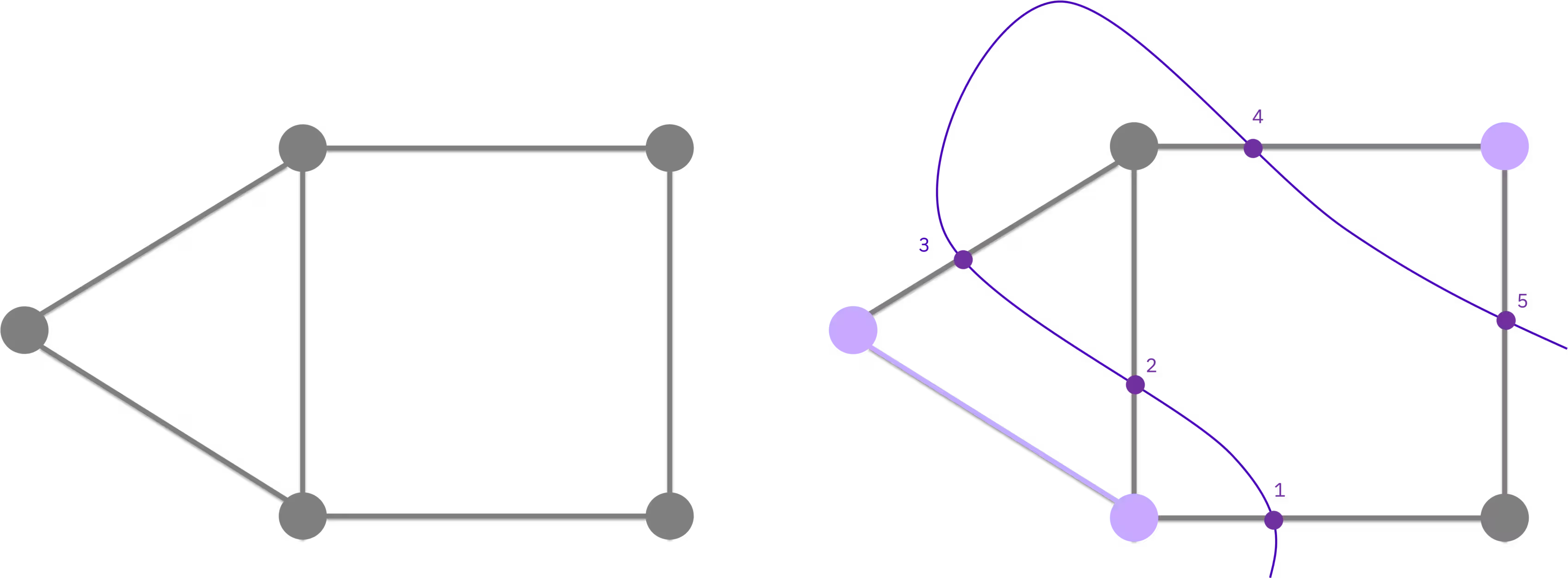
Des Minimum vo $f(x)$ in dem Fall liegt vor, wenn d'Anzahl da durch den Schnitt durchquertn Kantn maximal is. Wia mia sehn kenna, hod des no nix mit Quantencomputing z'toa. Mia müssn des Problem in was umformuliern, was a Quantencomputer verstehen ko. Initialisirts Euer Problem, indem mia an Graphen mit $n=5$ Knotn erstelln.

n = 5

graph = rx.PyGraph()
graph.add_nodes_from(np.arange(0, n, 1))
edge_list = [
    (0, 1, 1.0),
    (0, 2, 1.0),
    (0, 4, 1.0),
    (1, 2, 1.0),
    (2, 3, 1.0),
    (3, 4, 1.0),
]
graph.add_edges_from(edge_list)
draw_graph(graph, node_size=600, with_labels=True)

Schritt 1: Klassische Eingaben auf a Quantenproblem abbildn

Da erschte Schritt vom Pattern bestehd darin, des klassische Problem (Graph) auf quantenmechanische Schaltkreise und Operatoren abzubildn. Dazu san drei Hauptschritte z'unternehman:

1. Verwendung von ana Reihe mathematischer Umformulierungen, um des Problem mithilfe da Notation vo Quadratic Unconstrained Binary Optimization (QUBO) Problemen darzustelln.
2. Umformulierung vom Optimierungsproblem als Hamilton-Operator, für den da Grundzustand da Lösung entspricht, de d'Kostenfunktion minimiert.
3. Erstellung von am Quantenschaltkreis, wo den Grundzustand vo dem Hamilton-Operator über an Prozess ähnlich dem Quantum Annealing vorbereitet.

Hinweis: In da QAOA-Methodik woin mia letztendlich an Operator (Hamilton-Operator) ham, wo d'Kostenfunktion von unserm hybridn Algorithmus darstellt, sowie an parametrisierten Schaltkreis (Ansatz), wo Quantenzuständ mit Kandidatenlösungen für des Problem darstellt. Mia kenna aus dern Kandidatenzuständn sampln und sie dann mit da Kostenfunktion bewertn.

Graph → Optimierungsproblem

Da erschte Schritt da Abbildung is a Notationsänderung. Des Folgende drückt des Problem in QUBO-Notation aus:

$$\min_{x\in \{0, 1\}^n}x^T Q x,$$

wobei $Q$ a $n\times n$ Matrix reeller Zahlen is, $n$ da Anzahl da Knotn in Euerm Graphen entspricht, $x$ da obn eingeführte Vektor binärer Variablen is und $x^T$ d'Transponierte vom Vektor $x$ bezeichnet.

Maximize
 -2*x_0*x_1 - 2*x_0*x_2 - 2*x_0*x_4 - 2*x_1*x_2 - 2*x_2*x_3 - 2*x_3*x_4 + 3*x_0
 + 2*x_1 + 3*x_2 + 2*x_3 + 2*x_4

Subject to
  No constraints

  Binary variables (5)
    x_0 x_1 x_2 x_3 x_4

Optimierungsproblem → Hamilton-Operator

Mia kenna dann des QUBO-Problem als Hamilton-Operator umformuliern (do a Matrix, de d'Energie von am System darstellt):

$$H_C=\sum_{ij}Q_{ij}Z_iZ_j + \sum_i b_iZ_i.$$

Umformulierungsschritte vom QAOA-Problem zum Hamilton-Operator

Um z'demonstriern, wia des QAOA-Problem auf dera Weis umgschrieben wern ko, ersetzt mia zunächst d'binären Variablen $x_i$ durch an neien Satz vo Variablen $z_i\in\{-1, 1\}$ über

$$x_i = \frac{1-z_i}{2}.$$

Do kenna mia sehn, dass wenn $x_i$ gleich $0$ is, dann $z_i$ gleich $1$ sei muass. Wenn d'$x_i$ durch d'$z_i$ im Optimierungsproblem ($x^TQx$) ersetzt wern, ko a äquivalente Formulierung erhaitn wern.

$$x^TQx=\sum_{ij}Q_{ij}x_ix_j \\ =\frac{1}{4}\sum_{ij}Q_{ij}(1-z_i)(1-z_j) \\=\frac{1}{4}\sum_{ij}Q_{ij}z_iz_j-\frac{1}{4}\sum_{ij}(Q_{ij}+Q_{ji})z_i + \frac{n^2}{4}.$$

Wenn mia etzt $b_i=-\sum_{j}(Q_{ij}+Q_{ji})$ definiern, den Vorfaktor entfernern und den konstantn Term $n^2$ weglassn, kriagn mia d'zwoa äquivalentn Formulierungen vom selbn Optimierungsproblem.

$$\min_{x\in\{0,1\}^n} x^TQx\Longleftrightarrow \min_{z\in\{-1,1\}^n}z^TQz + b^Tz$$

Do hängt $b$ vo $Q$ ab. Beachts, dass mia zur Erlangung vo $z^TQz + b^Tz$ den Faktor 1/4 und an konstantn Offset vo $n^2$ wegglassn ham, de bei da Optimierung koa Rolle spieln.

Um etzt a Quantenformulierung vom Problem z'kriagn, hebn mia d'Variablen $z_i$ zu ana Pauli $Z$ Matrix, wia ana $2\times 2$ Matrix da Form

$$Z_i = \begin{pmatrix}1 & 0 \\ 0 & -1\end{pmatrix}.$$

Wenn mia dene Matrizen im obign Optimierungsproblem einsetzn, kriagn mia den folgendn Hamilton-Operator

$$H_C=\sum_{ij}Q_{ij}Z_iZ_j + \sum_i b_iZ_i.$$

Beachts a, dass d'$Z$ Matrizen in den Rechnenraum vom Quantencomputer einbettet san, des hoast in an Hilbert-Raum da Größe $2^n\times 2^n$. Daher solltets Terme wia $Z_iZ_j$ als des Tensorprodukt $Z_i\otimes Z_j$ verstehen, des in den $2^n\times 2^n$ Hilbert-Raum einbettet is. Zum Beispiel wird in am Problem mit fünf Entscheidungsvariablen da Term $Z_1Z_3$ als $I\otimes Z_3\otimes I\otimes Z_1\otimes I$ verstandn, wobei $I$ d'$2\times 2$ Einheitsmatrix is.

Deser Hamilton-Operator wird als Kostenfunktions-Hamilton-Operator bezeichnet. Er hod d'Eigenschaft, dass sei Grundzustand da Lösung entspricht, de d'Kostenfunktion $f(x)$ minimiert. Um Euer Optimierungsproblem zu lösen, müssn mia etzt den Grundzustand vo $H_C$ (oder an Zustand mit hoher Überlappung damit) auf dem Quantencomputer präpariern. Des Sampeln aus dem Zustand wird dann mit hoher Wahrscheinlichkeit d'Lösung zu $min~f(x)$ liefern. Schaugn mia uns etzt den Hamilton-Operator $H_C$ für des Max-Cut Problem an. Jedem Knotn vom Graphen wird a Qubit im Zustand $|0\rangle$ oder $|1\rangle$ zugeordnet, wobei da Wert d'Menge angibt, zu da da Knotn ghört. Des Ziel vom Problem is es, d'Anzahl da Kantn $(v_1, v_2)$ zu maximiern, für de $v_1 = |0\rangle$ und $v_2 = |1\rangle$ gilt, oder umgekehrt. Wenn mia den $Z$ Operator jedem Qubit zuordnn, wobei

$$Z|0\rangle = |0\rangle \qquad Z|1\rangle = -|1\rangle$$

dann ghört a Kante $(v_1, v_2)$ zum Schnitt, wenn da Eigenwert vo $(Z_1|v_1\rangle) \cdot (Z_2|v_2\rangle) = -1$ is; mit andern Wortn, d'mit $v_1$ und $v_2$ assoziierten Qubits san unterschiedlich. Ebenfalls ghört $(v_1, v_2)$ ned zum Schnitt, wenn da Eigenwert vo $(Z_1|v_1\rangle) \cdot (Z_2|v_2\rangle) = 1$ is. Beachts, dass uns da genaue Qubit-Zustand, wo jedem Knotn zugeordnet is, ned interessiert, sondern nur, ob sie über a Kante hinweg gleich san oder ned. Des Max-Cut-Problem verlangt vo uns, a Zuordnung da Qubits auf d'Knotn z'findn, so dass da Eigenwert vom folgendn Hamilton-Operator minimiert wird

$$H_C = \sum_{(i,j) \in e} Q_{ij} \cdot Z_i Z_j.$$

Mit andern Wortn, $b_i = 0$ für olle $i$ im Max-Cut-Problem. Da Wert vo $Q_{ij}$ bezeichnet des Gewicht da Kante. In dem Tutorial betrachtn mia an ungewichteten Graphen, des hoast $Q_{ij} = 1.0$ für olle $i, j$.

def build_max_cut_paulis(
    graph: rx.PyGraph,
) -> list[tuple[str, list[int], float]]:
    """Convert the graph to Pauli list.

    This function does the inverse of `build_max_cut_graph`
    """
    pauli_list = []
    for edge in list(graph.edge_list()):
        weight = graph.get_edge_data(edge[0], edge[1])
        pauli_list.append(("ZZ", [edge[0], edge[1]], weight))
    return pauli_list

max_cut_paulis = build_max_cut_paulis(graph)
cost_hamiltonian = SparsePauliOp.from_sparse_list(max_cut_paulis, n)
print("Cost Function Hamiltonian:", cost_hamiltonian)

Cost Function Hamiltonian: SparsePauliOp(['IIIZZ', 'IIZIZ', 'ZIIIZ', 'IIZZI', 'IZZII', 'ZZIII'],
              coeffs=[1.+0.j, 1.+0.j, 1.+0.j, 1.+0.j, 1.+0.j, 1.+0.j])

Hamilton-Operator → Quantenschaltkreis

Da Hamilton-Operator $H_C$ enthält d'Quantendefinition vo Euerm Problem. Etzt kenna mia an Quantenschaltkreis erstelln, wo dabei hilft, guade Lösungen vom Quantencomputer zu sampln. Da QAOA is inspiriert vom Quantum Annealing und wendet abwechselnde Schichtn von Operatorn im Quantenschaltkreis an.

D'allgemeine Idee bestehd darin, im Grundzustand von am bekanntn System z'beginnan, $H^{\otimes n}|0\rangle$ obn, und dann des System in den Grundzustand vom Kostenoperator z'steirn, an dem mia interessiert san. Des gschieht durch Anwendung da Operatorn $\exp\{-i\gamma_k H_C\}$ und $\exp\{-i\beta_k H_m\}$ mit Winkeln $\gamma_1,...,\gamma_p$ und $\beta_1,...,\beta_p~$.

Da vo Euch generierte Quantenschaltkreis is parametrisiert durch $\gamma_i$ und $\beta_i$, so dass mia verschiadene Werte vo $\gamma_i$ und $\beta_i$ ausprobirn und aus dem resultierenden Zustand sampln kenna.

In dem Fall wern mia a Beispiel mit ana QAOA-Schicht probirn, de zwoa Parameter enthält: $\gamma_1$ und $\beta_1$.

circuit = QAOAAnsatz(cost_operator=cost_hamiltonian, reps=2)
circuit.measure_all()

circuit.draw("mpl")

circuit.parameters

ParameterView([ParameterVectorElement(β[0]), ParameterVectorElement(β[1]), ParameterVectorElement(γ[0]), ParameterVectorElement(γ[1])])

Schritt 2: Problem für Quanten-Hardware-Ausführung optimiern

Da obige Schaltkreis enthält a Reihe vo Abstraktionen, de nützlich san, um über Quantenalgorithmen nachzudenken, aber auf da Hardware ned ausführbar san. Um auf ana QPU ausgführt wern z'kenna, muass da Schaltkreis a Reihe vo Operationen durchlaufn, de den Transpilations- oder Schaltkreis-Optimierungs-Schritt vom Pattern ausmachn.

D'Qiskit-Bibliothek bietet a Reihe vo Transpilations-Pässen, de a breite Palette vo Schaltkreistransformationen abdeckn. Mia müssn sicherstellen, dass Euer Schaltkreis für Euerern Zweck optimiert is.

D'Transpilation ko mehrere Schritte umfassn, wia zum Beispiel:

• Initiales Mapping da Qubits im Schaltkreis (wia Entscheidungsvariablen) auf physische Qubits auf dem Gerät.
• Unrolling da Anweisungen im Quantenschaltkreis zu den hardware-nativen Anweisungen, de des Backend verstehd.
• Routing beliebiger Qubits im Schaltkreis, wo interagiern, zu physischen Qubits, de benachbart zueinanda san.
• Fehlerunterdrückung durch Hinzufügn vo Einzelqubit-Gates zur Rauschunterdrückung mit dynamischer Entkopplung.

Weitere Informationen zur Transpilation findets in unserer Dokumentation.

Da folgende Code transformiert und optimiert den abstraktn Schaltkreis in a Format, des zur Ausführung auf am da über d'Cloud zugänglichn Geräte mit dem Qiskit IBM Runtime Service bereit is.

service = QiskitRuntimeService()
backend = service.least_busy(
    operational=True, simulator=False, min_num_qubits=127
)
print(backend)

# Create pass manager for transpilation
pm = generate_preset_pass_manager(optimization_level=3, backend=backend)

candidate_circuit = pm.run(circuit)
candidate_circuit.draw("mpl", fold=False, idle_wires=False)

<IBMBackend('test_heron_pok_1')>

Schritt 3: Ausführung mit Qiskit Primitives

Im QAOA-Workflow wern d'optimalen QAOA-Parameter in ana iterativen Optimierungsschleife gfundn, de a Reihe vo Schaltkreisbewertungen ausführt und an klassischn Optimierer verwendt, um d'optimalen $\beta_k$ und $\gamma_k$ Parameter z'findn. Dese Ausführungsschleife wird über d'folgendn Schritte ausgführt:

1. Definierung da initialen Parameter
2. Instanziierung von ana neien Session, de d'Optimierungsschleife und des Primitive enthält, wo zum Sampln vom Schaltkreis verwendt wird
3. Sobald a optimaler Parametersatz gfundn is, führts den Schaltkreis a letztns Mal aus, um a finale Verteilung z'kriagn, de im Post-Processing-Schritt verwendt wird.

Schaltkreis mit initialen Parametern definiern

Mia fanng mit willkürlich gwahltn Parametern an.

initial_gamma = np.pi
initial_beta = np.pi / 2
init_params = [initial_beta, initial_beta, initial_gamma, initial_gamma]

Backend und Ausführungs-Primitive definiern

Verwendts d'Qiskit Runtime Primitives, um mit IBM® Backends z'interagiern. D'zwoa Primitives san Sampler und Estimator, und d'Wahl vom Primitive hängt davon ob, welche Art vo Messung mia auf dem Quantencomputer ausführn woin. Für d'Minimierung vo $H_C$ verwendts den Estimator, weil d'Messung da Kostenfunktion einfach da Erwartungswert vo $\langle H_C \rangle$ is.

Ausführn

D'Primitives bietn a Vielzahl vo Ausführungsmodi zur Planung vo Workloads auf Quantengeräten, und a QAOA-Workflow läuft iterativ in ana Session.

Mia kenna d'sampler-basierte Kostenfunktion in d'SciPy-Minimierungsroutine eistecka, um d'optimalen Parameter z'findn.

def cost_func_estimator(params, ansatz, hamiltonian, estimator):
    # transform the observable defined on virtual qubits to
    # an observable defined on all physical qubits
    isa_hamiltonian = hamiltonian.apply_layout(ansatz.layout)

    pub = (ansatz, isa_hamiltonian, params)
    job = estimator.run([pub])

    results = job.result()[0]
    cost = results.data.evs

    objective_func_vals.append(cost)

    return cost

objective_func_vals = []  # Global variable
with Session(backend=backend) as session:
    # If using qiskit-ibm-runtime<0.24.0, change `mode=` to `session=`
    estimator = Estimator(mode=session)
    estimator.options.default_shots = 1000

    # Set simple error suppression/mitigation options
    estimator.options.dynamical_decoupling.enable = True
    estimator.options.dynamical_decoupling.sequence_type = "XY4"
    estimator.options.twirling.enable_gates = True
    estimator.options.twirling.num_randomizations = "auto"

    result = minimize(
        cost_func_estimator,
        init_params,
        args=(candidate_circuit, cost_hamiltonian, estimator),
        method="COBYLA",
        tol=1e-2,
    )
    print(result)

message: Return from COBYLA because the trust region radius reaches its lower bound.
 success: True
  status: 0
     fun: -1.6295230263157894
       x: [ 1.530e+00  1.439e+00  4.071e+00  4.434e+00]
    nfev: 26
   maxcv: 0.0

Da Optimierer konnte d'Kosten reduziern und bessere Parameter für den Schaltkreis findn.

plt.figure(figsize=(12, 6))
plt.plot(objective_func_vals)
plt.xlabel("Iteration")
plt.ylabel("Cost")
plt.show()

Sobald mia d'optimalen Parameter für den Schaltkreis gfundn ham, kenna mia dene Parameter zuweisn und d'mit den optimierten Parametern erhaltene finale Verteilung sampln. Do sollt des Sampler Primitive verwendt wern, weil es d'Wahrscheinlichkeitsverteilung vo Bitstring-Messungen is, de dem optimalen Schnitt vom Graphen entsprechn.

Hinweis: Des bedeutet, an Quantenzustand $\psi$ im Computer z'präpariern und ihn dann z'messn. A Messung wird den Zustand in an einzelnen Berechnungsbasiszustand kollabiern - zum Beispiel 010101110000... - wo ana Kandidatenlösung $x$ für unser ursprünglichs Optimierungsproblem ($\max f(x)$ oder $\min f(x)$ je nach Aufgabe) entspricht.

optimized_circuit = candidate_circuit.assign_parameters(result.x)
optimized_circuit.draw("mpl", fold=False, idle_wires=False)

# If using qiskit-ibm-runtime<0.24.0, change `mode=` to `backend=`
sampler = Sampler(mode=backend)
sampler.options.default_shots = 10000

# Set simple error suppression/mitigation options
sampler.options.dynamical_decoupling.enable = True
sampler.options.dynamical_decoupling.sequence_type = "XY4"
sampler.options.twirling.enable_gates = True
sampler.options.twirling.num_randomizations = "auto"

pub = (optimized_circuit,)
job = sampler.run([pub], shots=int(1e4))
counts_int = job.result()[0].data.meas.get_int_counts()
counts_bin = job.result()[0].data.meas.get_counts()
shots = sum(counts_int.values())
final_distribution_int = {key: val / shots for key, val in counts_int.items()}
final_distribution_bin = {key: val / shots for key, val in counts_bin.items()}
print(final_distribution_int)

{28: 0.0328, 11: 0.0343, 2: 0.0296, 25: 0.0308, 16: 0.0303, 27: 0.0302, 13: 0.0323, 7: 0.0312, 4: 0.0296, 9: 0.0295, 26: 0.0321, 30: 0.031, 23: 0.0324, 31: 0.0303, 21: 0.0335, 15: 0.0317, 12: 0.0309, 29: 0.0297, 3: 0.0313, 5: 0.0312, 6: 0.0274, 10: 0.0329, 22: 0.0353, 0: 0.0315, 20: 0.0326, 8: 0.0322, 14: 0.0306, 17: 0.0295, 18: 0.0279, 1: 0.0325, 24: 0.0334, 19: 0.0295}

Schritt 4: Nachbearbeitung und Rückgabe vom Ergebnis im gwünschten klassischn Format

Da Nachbearbeitungsschritt interpretierd d'Sampling-Ausgabe, um a Lösung für Euer ursprünglichs Problem zurückzugeben. In dem Fall san mia an dem Bitstring mit da höchstn Wahrscheinlichkeit interessiert, weil deser den optimalen Schnitt bestimmt. D'Symmetrien im Problem erlaubn vier mögliche Lösungen, und da Sampling-Prozess wird a davon mit ana etwas höhern Wahrscheinlichkeit zurückgebn, aber mia kenna in da untn dargestelltn Verteilung sehn, dass vier da Bitstrings deutlich wahrscheinlicher san als da Rest.

# auxiliary functions to sample most likely bitstring
def to_bitstring(integer, num_bits):
    result = np.binary_repr(integer, width=num_bits)
    return [int(digit) for digit in result]

keys = list(final_distribution_int.keys())
values = list(final_distribution_int.values())
most_likely = keys[np.argmax(np.abs(values))]
most_likely_bitstring = to_bitstring(most_likely, len(graph))
most_likely_bitstring.reverse()

print("Result bitstring:", most_likely_bitstring)

Result bitstring: [0, 1, 1, 0, 1]

matplotlib.rcParams.update({"font.size": 10})
final_bits = final_distribution_bin
values = np.abs(list(final_bits.values()))
top_4_values = sorted(values, reverse=True)[:4]
positions = []
for value in top_4_values:
    positions.append(np.where(values == value)[0])
fig = plt.figure(figsize=(11, 6))
ax = fig.add_subplot(1, 1, 1)
plt.xticks(rotation=45)
plt.title("Result Distribution")
plt.xlabel("Bitstrings (reversed)")
plt.ylabel("Probability")
ax.bar(list(final_bits.keys()), list(final_bits.values()), color="tab:grey")
for p in positions:
    ax.get_children()[int(p[0])].set_color("tab:purple")
plt.show()

Besten Schnitt visualisiern

Aus dem optimalen Bitstring kenna mia dann den Schnitt auf dem ursprünglichn Graphen visualisiern.

# auxiliary function to plot graphs
def plot_result(G, x):
    colors = ["tab:grey" if i == 0 else "tab:purple" for i in x]
    pos, _default_axes = rx.spring_layout(G), plt.axes(frameon=True)
    rx.visualization.mpl_draw(
        G, node_color=colors, node_size=100, alpha=0.8, pos=pos
    )

plot_result(graph, most_likely_bitstring)

Und berechnt den Wert vom Schnitt:

def evaluate_sample(x: Sequence[int], graph: rx.PyGraph) -> float:
    assert len(x) == len(
        list(graph.nodes())
    ), "The length of x must coincide with the number of nodes in the graph."
    return sum(
        x[u] * (1 - x[v]) + x[v] * (1 - x[u])
        for u, v in list(graph.edge_list())
    )

cut_value = evaluate_sample(most_likely_bitstring, graph)
print("The value of the cut is:", cut_value)

The value of the cut is: 5

Teil II. Skalierng auffe!

Mia ham Zugang zu vüln Gerätn mit über 100 Qubits auf da IBM Quantum® Platform. Wählts oas aus, auf dem Max-Cut auf am 100-Knoten-gewichteten Graphen glöst wern soll. Des is a Problem im "Utility-Maßstab". D'Schritte zum Aufbau vom Workflow san d'gleichen wia obn, jedoch mit am vül größern Graphen.

n = 100  # Number of nodes in graph
graph_100 = rx.PyGraph()
graph_100.add_nodes_from(np.arange(0, n, 1))
elist = []
for edge in backend.coupling_map:
    if edge[0] < n and edge[1] < n:
        elist.append((edge[0], edge[1], 1.0))
graph_100.add_edges_from(elist)
draw_graph(graph_100, node_size=200, with_labels=True, width=1)

Schritt 1: Klassische Eingaben auf a Quantenproblem abbildn

Graph → Hamilton-Operator

Konvertierst zunächst den Graphen, den mia lösen woin, direkt in an Hamilton-Operator, wo für QAOA geignet is.

max_cut_paulis_100 = build_max_cut_paulis(graph_100)

cost_hamiltonian_100 = SparsePauliOp.from_sparse_list(max_cut_paulis_100, 100)
print("Cost Function Hamiltonian:", cost_hamiltonian_100)

Cost Function Hamiltonian: SparsePauliOp(['IIIIIIIIIIIIIIIIIIIIIIIIIIIIIIIIIIIIIIIIIIIIIIIIIIIIIIIIIIIIIIIIIIIIIIIIIIIIIIIIIIIIIIIIIIIIIIIIIIZZ', 'IIIIIIIIIIIIIIIIIIIIIIIIIIIIIIIIIIIIIIIIIIIIIIIIIIIIIIIIIIIIIIIIIIIIIIIIIIIIIIIIIIIIIIIIIIIIIIIIIIZZ', 'IIIIIIIIIIIIIIIIIIIIIIIIIIIIIIIIIIIIIIIIIIIIIIIIIIIIIIIIIIIIIIIIIIIIIIIIIIIIIIIIIIIIIIIIIIIIIIIIIZZI', 'IIIIIIIIIIIIIIIIIIIIIIIIIIIIIIIIIIIIIIIIIIIIIIIIIIIIIIIIIIIIIIIIIIIIIIIIIIIIIIIIIIIIIIIIIIIIIIIIIZZI', 'IIIIIIIIIIIIIIIIIIIIIIIIIIIIIIIIIIIIIIIIIIIIIIIIIIIIIIIIIIIIIIIIIIIIIIIIIIIIIIIIIIIIIIIIIIIIIIIIZZII', 'IIIIIIIIIIIIIIIIIIIIIIIIIIIIIIIIIIIIIIIIIIIIIIIIIIIIIIIIIIIIIIIIIIIIIIIIIIIIIIIIIIIIIIIIIIIIIIIIZZII', 'IIIIIIIIIIIIIIIIIIIIIIIIIIIIIIIIIIIIIIIIIIIIIIIIIIIIIIIIIIIIIIIIIIIIIIIIIIIIIIIIIIIIIIIIIIIIIIIZZIII', 'IIIIIIIIIIIIIIIIIIIIIIIIIIIIIIIIIIIIIIIIIIIIIIIIIIIIIIIIIIIIIIIIIIIIIIIIIIIIIIIIIIIZIIIIIIIIIIIIZIII', 'IIIIIIIIIIIIIIIIIIIIIIIIIIIIIIIIIIIIIIIIIIIIIIIIIIIIIIIIIIIIIIIIIIIIIIIIIIIIIIIIIIIIIIIIIIIIIIIZZIII', 'IIIIIIIIIIIIIIIIIIIIIIIIIIIIIIIIIIIIIIIIIIIIIIIIIIIIIIIIIIIIIIIIIIIIIIIIIIIIIIIIIIIIIIIIIIIIIIZZIIII', 'IIIIIIIIIIIIIIIIIIIIIIIIIIIIIIIIIIIIIIIIIIIIIIIIIIIIIIIIIIIIIIIIIIIIIIIIIIIIIIIIIIIIIIIIIIIIIIZZIIII', 'IIIIIIIIIIIIIIIIIIIIIIIIIIIIIIIIIIIIIIIIIIIIIIIIIIIIIIIIIIIIIIIIIIIIIIIIIIIIIIIIIIIIIIIIIIIIIZZIIIII', 'IIIIIIIIIIIIIIIIIIIIIIIIIIIIIIIIIIIIIIIIIIIIIIIIIIIIIIIIIIIIIIIIIIIIIIIIIIIIIIIIIIIIIIIIIIIIIZZIIIII', 'IIIIIIIIIIIIIIIIIIIIIIIIIIIIIIIIIIIIIIIIIIIIIIIIIIIIIIIIIIIIIIIIIIIIIIIIIIIIIIIIIIIIIIIIIIIIZZIIIIII', 'IIIIIIIIIIIIIIIIIIIIIIIIIIIIIIIIIIIIIIIIIIIIIIIIIIIIIIIIIIIIIIIIIIIIIIIIIIIIIIIIIIIIIIIIIIIIZZIIIIII', 'IIIIIIIIIIIIIIIIIIIIIIIIIIIIIIIIIIIIIIIIIIIIIIIIIIIIIIIIIIIIIIIIIIIIIIIIIIIIIIIIIIIIIIIIIIIZZIIIIIII', 'IIIIIIIIIIIIIIIIIIIIIIIIIIIIIIIIIIIIIIIIIIIIIIIIIIIIIIIIIIIIIIIIIIIIIIIIIIIIIIIIIIZIIIIIIIIIZIIIIIII', 'IIIIIIIIIIIIIIIIIIIIIIIIIIIIIIIIIIIIIIIIIIIIIIIIIIIIIIIIIIIIIIIIIIIIIIIIIIIIIIIIIIIIIIIIIIIZZIIIIIII', 'IIIIIIIIIIIIIIIIIIIIIIIIIIIIIIIIIIIIIIIIIIIIIIIIIIIIIIIIIIIIIIIIIIIIIIIIIIIIIIIIIIIIIIIIIIZZIIIIIIII', 'IIIIIIIIIIIIIIIIIIIIIIIIIIIIIIIIIIIIIIIIIIIIIIIIIIIIIIIIIIIIIIIIIIIIIIIIIIIIIIIIIIIIIIIIIIZZIIIIIIII', 'IIIIIIIIIIIIIIIIIIIIIIIIIIIIIIIIIIIIIIIIIIIIIIIIIIIIIIIIIIIIIIIIIIIIIIIIIIIIIIIIIIIIIIIIIZZIIIIIIIII', 'IIIIIIIIIIIIIIIIIIIIIIIIIIIIIIIIIIIIIIIIIIIIIIIIIIIIIIIIIIIIIIIIIIIIIIIIIIIIIIIIIIIIIIIIIZZIIIIIIIII', 'IIIIIIIIIIIIIIIIIIIIIIIIIIIIIIIIIIIIIIIIIIIIIIIIIIIIIIIIIIIIIIIIIIIIIIIIIIIIIIIIIIIIIIIIZZIIIIIIIIII', 'IIIIIIIIIIIIIIIIIIIIIIIIIIIIIIIIIIIIIIIIIIIIIIIIIIIIIIIIIIIIIIIIIIIIIIIIIIIIIIIIIIIIIIIIZZIIIIIIIIII', 'IIIIIIIIIIIIIIIIIIIIIIIIIIIIIIIIIIIIIIIIIIIIIIIIIIIIIIIIIIIIIIIIIIIIIIIIIIIIIIIIIIIIIIIZZIIIIIIIIIII', 'IIIIIIIIIIIIIIIIIIIIIIIIIIIIIIIIIIIIIIIIIIIIIIIIIIIIIIIIIIIIIIIIIIIIIIIIIIIIIIIIIZIIIIIIZIIIIIIIIIII', 'IIIIIIIIIIIIIIIIIIIIIIIIIIIIIIIIIIIIIIIIIIIIIIIIIIIIIIIIIIIIIIIIIIIIIIIIIIIIIIIIIIIIIIIZZIIIIIIIIIII', 'IIIIIIIIIIIIIIIIIIIIIIIIIIIIIIIIIIIIIIIIIIIIIIIIIIIIIIIIIIIIIIIIIIIIIIIIIIIIIIIIIIIIIIZZIIIIIIIIIIII', 'IIIIIIIIIIIIIIIIIIIIIIIIIIIIIIIIIIIIIIIIIIIIIIIIIIIIIIIIIIIIIIIIIIIIIIIIIIIIIIIIIIIIIIZZIIIIIIIIIIII', 'IIIIIIIIIIIIIIIIIIIIIIIIIIIIIIIIIIIIIIIIIIIIIIIIIIIIIIIIIIIIIIIIIIIIIIIIIIIIIIIIIIIIIZZIIIIIIIIIIIII', 'IIIIIIIIIIIIIIIIIIIIIIIIIIIIIIIIIIIIIIIIIIIIIIIIIIIIIIIIIIIIIIIIIIIIIIIIIIIIIIIIIIIIIZZIIIIIIIIIIIII', 'IIIIIIIIIIIIIIIIIIIIIIIIIIIIIIIIIIIIIIIIIIIIIIIIIIIIIIIIIIIIIIIIIIIIIIIIIIIIIIIIIIIIZZIIIIIIIIIIIIII', 'IIIIIIIIIIIIIIIIIIIIIIIIIIIIIIIIIIIIIIIIIIIIIIIIIIIIIIIIIIIIIIIIIIIIIIIIIIIIIIIIIIIIZZIIIIIIIIIIIIII', 'IIIIIIIIIIIIIIIIIIIIIIIIIIIIIIIIIIIIIIIIIIIIIIIIIIIIIIIIIIIIIIIIIIIIIIIIIIIIIIIIZIIIZIIIIIIIIIIIIIII', 'IIIIIIIIIIIIIIIIIIIIIIIIIIIIIIIIIIIIIIIIIIIIIIIIIIIIIIIIIIIIIIIIIIIIIIIIIIIIIIIIIIIZIIIIIIIIIIIIZIII', 'IIIIIIIIIIIIIIIIIIIIIIIIIIIIIIIIIIIIIIIIIIIIIIIIIIIIIIIIIIIIIIIIIIIIIIIIIIIIZIIIIIIZIIIIIIIIIIIIIIII', 'IIIIIIIIIIIIIIIIIIIIIIIIIIIIIIIIIIIIIIIIIIIIIIIIIIIIIIIIIIIIIIIIIIIIIIIIIIIIIIIIIIZIIIIIIIIIZIIIIIII', 'IIIIIIIIIIIIIIIIIIIIIIIIIIIIIIIIIIIIIIIIIIIIIIIIIIIIIIIIIIIIIIIIIIIIIIIIZIIIIIIIIIZIIIIIIIIIIIIIIIII', 'IIIIIIIIIIIIIIIIIIIIIIIIIIIIIIIIIIIIIIIIIIIIIIIIIIIIIIIIIIIIIIIIIIIIIIIIIIIIIIIIIZIIIIIIZIIIIIIIIIII', 'IIIIIIIIIIIIIIIIIIIIIIIIIIIIIIIIIIIIIIIIIIIIIIIIIIIIIIIIIIIIIIIIIIIIZIIIIIIIIIIIIZIIIIIIIIIIIIIIIIII', 'IIIIIIIIIIIIIIIIIIIIIIIIIIIIIIIIIIIIIIIIIIIIIIIIIIIIIIIIIIIIIIIIIIIIIIIIIIIIIIIIZIIIZIIIIIIIIIIIIIII', 'IIIIIIIIIIIIIIIIIIIIIIIIIIIIIIIIIIIIIIIIIIIIIIIIIIIIIIIIIIIIIIIIZIIIIIIIIIIIIIIIZIIIIIIIIIIIIIIIIIII', 'IIIIIIIIIIIIIIIIIIIIIIIIIIIIIIIIIIIIIIIIIIIIIIIIIIIIIIIIIIIIIIIIIIIIIIIIIIIIIIZZIIIIIIIIIIIIIIIIIIII', 'IIIIIIIIIIIIIIIIIIIIIIIIIIIIIIIIIIIIIIIIIIIIIIIIIIIIIIIIIIIIIIIIIIIIIIIIIIIIIIZZIIIIIIIIIIIIIIIIIIII', 'IIIIIIIIIIIIIIIIIIIIIIIIIIIIIIIIIIIIIIIIIIIIIIIIIIIIIIIIIIIIIIIIIIIIIIIIIIIIIZZIIIIIIIIIIIIIIIIIIIII', 'IIIIIIIIIIIIIIIIIIIIIIIIIIIIIIIIIIIIIIIIIIIIIIIIIIIIIIIIIIIIIIIZIIIIIIIIIIIIIIZIIIIIIIIIIIIIIIIIIIII', 'IIIIIIIIIIIIIIIIIIIIIIIIIIIIIIIIIIIIIIIIIIIIIIIIIIIIIIIIIIIIIIIIIIIIIIIIIIIIIZZIIIIIIIIIIIIIIIIIIIII', 'IIIIIIIIIIIIIIIIIIIIIIIIIIIIIIIIIIIIIIIIIIIIIIIIIIIIIIIIIIIIIIIIIIIIIIIIIIIIZZIIIIIIIIIIIIIIIIIIIIII', 'IIIIIIIIIIIIIIIIIIIIIIIIIIIIIIIIIIIIIIIIIIIIIIIIIIIIIIIIIIIIIIIIIIIIIIIIIIIIZIIIIIIZIIIIIIIIIIIIIIII', 'IIIIIIIIIIIIIIIIIIIIIIIIIIIIIIIIIIIIIIIIIIIIIIIIIIIIIIIIIIIIIIIIIIIIIIIIIIIIZZIIIIIIIIIIIIIIIIIIIIII', 'IIIIIIIIIIIIIIIIIIIIIIIIIIIIIIIIIIIIIIIIIIIIIIIIIIIIIIIIIIIIIIIIIIIIIIIIIIIZZIIIIIIIIIIIIIIIIIIIIIII', 'IIIIIIIIIIIIIIIIIIIIIIIIIIIIIIIIIIIIIIIIIIIIIIIIIIIIIIIIIIIIIIIIIIIIIIIIIIIZZIIIIIIIIIIIIIIIIIIIIIII', 'IIIIIIIIIIIIIIIIIIIIIIIIIIIIIIIIIIIIIIIIIIIIIIIIIIIIIIIIIIIIIIIIIIIIIIIIIIZZIIIIIIIIIIIIIIIIIIIIIIII', 'IIIIIIIIIIIIIIIIIIIIIIIIIIIIIIIIIIIIIIIIIIIIIIIIIIIIIIIIIIIIIIIIIIIIIIIIIIZZIIIIIIIIIIIIIIIIIIIIIIII', 'IIIIIIIIIIIIIIIIIIIIIIIIIIIIIIIIIIIIIIIIIIIIIIIIIIIIIIIIIIIIIIIIIIIIIIIIIZZIIIIIIIIIIIIIIIIIIIIIIIII', 'IIIIIIIIIIIIIIIIIIIIIIIIIIIIIIIIIIIIIIIIIIIIIIIIIIIIIIIIIIIIIIZIIIIIIIIIIIZIIIIIIIIIIIIIIIIIIIIIIIII', 'IIIIIIIIIIIIIIIIIIIIIIIIIIIIIIIIIIIIIIIIIIIIIIIIIIIIIIIIIIIIIIIIIIIIIIIIIZZIIIIIIIIIIIIIIIIIIIIIIIII', 'IIIIIIIIIIIIIIIIIIIIIIIIIIIIIIIIIIIIIIIIIIIIIIIIIIIIIIIIIIIIIIIIIIIIIIIIZZIIIIIIIIIIIIIIIIIIIIIIIIII', 'IIIIIIIIIIIIIIIIIIIIIIIIIIIIIIIIIIIIIIIIIIIIIIIIIIIIIIIIIIIIIIIIIIIIIIIIZIIIIIIIIIZIIIIIIIIIIIIIIIII', 'IIIIIIIIIIIIIIIIIIIIIIIIIIIIIIIIIIIIIIIIIIIIIIIIIIIIIIIIIIIIIIIIIIIIIIIIZZIIIIIIIIIIIIIIIIIIIIIIIIII', 'IIIIIIIIIIIIIIIIIIIIIIIIIIIIIIIIIIIIIIIIIIIIIIIIIIIIIIIIIIIIIIIIIIIIIIIZZIIIIIIIIIIIIIIIIIIIIIIIIIII', 'IIIIIIIIIIIIIIIIIIIIIIIIIIIIIIIIIIIIIIIIIIIIIIIIIIIIIIIIIIIIIIIIIIIIIIIZZIIIIIIIIIIIIIIIIIIIIIIIIIII', 'IIIIIIIIIIIIIIIIIIIIIIIIIIIIIIIIIIIIIIIIIIIIIIIIIIIIIIIIIIIIIIIIIIIIIIZZIIIIIIIIIIIIIIIIIIIIIIIIIIII', 'IIIIIIIIIIIIIIIIIIIIIIIIIIIIIIIIIIIIIIIIIIIIIIIIIIIIIIIIIIIIIIIIIIIIIIZZIIIIIIIIIIIIIIIIIIIIIIIIIIII', 'IIIIIIIIIIIIIIIIIIIIIIIIIIIIIIIIIIIIIIIIIIIIIIIIIIIIIIIIIIIIIIIIIIIIIZZIIIIIIIIIIIIIIIIIIIIIIIIIIIII', 'IIIIIIIIIIIIIIIIIIIIIIIIIIIIIIIIIIIIIIIIIIIIIIIIIIIIIIIIIIIIIZIIIIIIIIZIIIIIIIIIIIIIIIIIIIIIIIIIIIII', 'IIIIIIIIIIIIIIIIIIIIIIIIIIIIIIIIIIIIIIIIIIIIIIIIIIIIIIIIIIIIIIIIIIIIIZZIIIIIIIIIIIIIIIIIIIIIIIIIIIII', 'IIIIIIIIIIIIIIIIIIIIIIIIIIIIIIIIIIIIIIIIIIIIIIIIIIIIIIIIIIIIIIIIIIIIZZIIIIIIIIIIIIIIIIIIIIIIIIIIIIII', 'IIIIIIIIIIIIIIIIIIIIIIIIIIIIIIIIIIIIIIIIIIIIIIIIIIIIIIIIIIIIIIIIIIIIZIIIIIIIIIIIIZIIIIIIIIIIIIIIIIII', 'IIIIIIIIIIIIIIIIIIIIIIIIIIIIIIIIIIIIIIIIIIIIIIIIIIIIIIIIIIIIIIIIIIIIZZIIIIIIIIIIIIIIIIIIIIIIIIIIIIII', 'IIIIIIIIIIIIIIIIIIIIIIIIIIIIIIIIIIIIIIIIIIIIIIIIIIIIIIIIIIIIIIIIIIIZZIIIIIIIIIIIIIIIIIIIIIIIIIIIIIII', 'IIIIIIIIIIIIIIIIIIIIIIIIIIIIIIIIIIIIIIIIIIIIIIIIIIIIIIIIIIIIIIIIIIIZZIIIIIIIIIIIIIIIIIIIIIIIIIIIIIII', 'IIIIIIIIIIIIIIIIIIIIIIIIIIIIIIIIIIIIIIIIIIIIIIIIIIIIIIIIIIIIIIIIIIZZIIIIIIIIIIIIIIIIIIIIIIIIIIIIIIII', 'IIIIIIIIIIIIIIIIIIIIIIIIIIIIIIIIIIIIIIIIIIIIIIIIIIIIIIIIIIIIIIIIIIZZIIIIIIIIIIIIIIIIIIIIIIIIIIIIIIII', 'IIIIIIIIIIIIIIIIIIIIIIIIIIIIIIIIIIIIIIIIIIIIIIIIIIIIIIIIIIIIIIIIIZZIIIIIIIIIIIIIIIIIIIIIIIIIIIIIIIII', 'IIIIIIIIIIIIIIIIIIIIIIIIIIIIIIIIIIIIIIIIIIIIIIIIIIIIIIIIIIIIZIIIIIZIIIIIIIIIIIIIIIIIIIIIIIIIIIIIIIII', 'IIIIIIIIIIIIIIIIIIIIIIIIIIIIIIIIIIIIIIIIIIIIIIIIIIIIIIIIIIIIIIIIIZZIIIIIIIIIIIIIIIIIIIIIIIIIIIIIIIII', 'IIIIIIIIIIIIIIIIIIIIIIIIIIIIIIIIIIIIIIIIIIIIIIIIIIIIIIIIIIIIIIIIZZIIIIIIIIIIIIIIIIIIIIIIIIIIIIIIIIII', 'IIIIIIIIIIIIIIIIIIIIIIIIIIIIIIIIIIIIIIIIIIIIIIIIIIIIIIIIIIIIIIIIZIIIIIIIIIIIIIIIZIIIIIIIIIIIIIIIIIII', 'IIIIIIIIIIIIIIIIIIIIIIIIIIIIIIIIIIIIIIIIIIIIIIIIIIIIIIIIIIIIIIIIZZIIIIIIIIIIIIIIIIIIIIIIIIIIIIIIIIII', 'IIIIIIIIIIIIIIIIIIIIIIIIIIIIIIIIIIIIIIIIIIIIIIIIIIIIIIIIIIIIIIIZIIIIIIIIIIIIIIZIIIIIIIIIIIIIIIIIIIII', 'IIIIIIIIIIIIIIIIIIIIIIIIIIIIIIIIIIIIIIIIIIIIIIIIIIIIIIIIIIZIIIIZIIIIIIIIIIIIIIIIIIIIIIIIIIIIIIIIIIII', 'IIIIIIIIIIIIIIIIIIIIIIIIIIIIIIIIIIIIIIIIIIIIIIIIIIIIIIIIIIIIIIZIIIIIIIIIIIZIIIIIIIIIIIIIIIIIIIIIIIII', 'IIIIIIIIIIIIIIIIIIIIIIIIIIIIIIIIIIIIIIIIIIIIIIIIIIIIIIZIIIIIIIZIIIIIIIIIIIIIIIIIIIIIIIIIIIIIIIIIIIII', 'IIIIIIIIIIIIIIIIIIIIIIIIIIIIIIIIIIIIIIIIIIIIIIIIIIIIIIIIIIIIIZIIIIIIIIZIIIIIIIIIIIIIIIIIIIIIIIIIIIII', 'IIIIIIIIIIIIIIIIIIIIIIIIIIIIIIIIIIIIIIIIIIIIIIIIIIZIIIIIIIIIIZIIIIIIIIIIIIIIIIIIIIIIIIIIIIIIIIIIIIII', 'IIIIIIIIIIIIIIIIIIIIIIIIIIIIIIIIIIIIIIIIIIIIIIIIIIIIIIIIIIIIZIIIIIZIIIIIIIIIIIIIIIIIIIIIIIIIIIIIIIII', 'IIIIIIIIIIIIIIIIIIIIIIIIIIIIIIIIIIIIIIIIIIIIIIZIIIIIIIIIIIIIZIIIIIIIIIIIIIIIIIIIIIIIIIIIIIIIIIIIIIII', 'IIIIIIIIIIIIIIIIIIIIIIIIIIIIIIIIIIIIIIIIIIIIIIIIIIIIIIIIIIZZIIIIIIIIIIIIIIIIIIIIIIIIIIIIIIIIIIIIIIII', 'IIIIIIIIIIIIIIIIIIIIIIIIIIIIIIIIIIIIIIIIIIIIIIIIIIIIIIIIIIZIIIIZIIIIIIIIIIIIIIIIIIIIIIIIIIIIIIIIIIII', 'IIIIIIIIIIIIIIIIIIIIIIIIIIIIIIIIIIIIIIIIIIIIIIIIIIIIIIIIIIZZIIIIIIIIIIIIIIIIIIIIIIIIIIIIIIIIIIIIIIII', 'IIIIIIIIIIIIIIIIIIIIIIIIIIIIIIIIIIIIIIIIIIIIIIIIIIIIIIIIIZZIIIIIIIIIIIIIIIIIIIIIIIIIIIIIIIIIIIIIIIII', 'IIIIIIIIIIIIIIIIIIIIIIIIIIIIIIIIIIIIIIIIIIIIIIIIIIIIIIIIIZZIIIIIIIIIIIIIIIIIIIIIIIIIIIIIIIIIIIIIIIII', 'IIIIIIIIIIIIIIIIIIIIIIIIIIIIIIIIIIIIIIIIIIIIIIIIIIIIIIIIZZIIIIIIIIIIIIIIIIIIIIIIIIIIIIIIIIIIIIIIIIII', 'IIIIIIIIIIIIIIIIIIIIIIIIIIIIIIIIIIIIIIIIIIIIIIIIIIIIIIIIZZIIIIIIIIIIIIIIIIIIIIIIIIIIIIIIIIIIIIIIIIII', 'IIIIIIIIIIIIIIIIIIIIIIIIIIIIIIIIIIIIIIIIIIIIIIIIIIIIIIIZZIIIIIIIIIIIIIIIIIIIIIIIIIIIIIIIIIIIIIIIIIII', 'IIIIIIIIIIIIIIIIIIIIIIIIIIIIIIIIIIIIIIIIIIIZIIIIIIIIIIIIZIIIIIIIIIIIIIIIIIIIIIIIIIIIIIIIIIIIIIIIIIII', 'IIIIIIIIIIIIIIIIIIIIIIIIIIIIIIIIIIIIIIIIIIIIIIIIIIIIIIIZZIIIIIIIIIIIIIIIIIIIIIIIIIIIIIIIIIIIIIIIIIII', 'IIIIIIIIIIIIIIIIIIIIIIIIIIIIIIIIIIIIIIIIIIIIIIIIIIIIIIZZIIIIIIIIIIIIIIIIIIIIIIIIIIIIIIIIIIIIIIIIIIII', 'IIIIIIIIIIIIIIIIIIIIIIIIIIIIIIIIIIIIIIIIIIIIIIIIIIIIIIZIIIIIIIZIIIIIIIIIIIIIIIIIIIIIIIIIIIIIIIIIIIII', 'IIIIIIIIIIIIIIIIIIIIIIIIIIIIIIIIIIIIIIIIIIIIIIIIIIIIIIZZIIIIIIIIIIIIIIIIIIIIIIIIIIIIIIIIIIIIIIIIIIII', 'IIIIIIIIIIIIIIIIIIIIIIIIIIIIIIIIIIIIIIIIIIIIIIIIIIIIIZZIIIIIIIIIIIIIIIIIIIIIIIIIIIIIIIIIIIIIIIIIIIII', 'IIIIIIIIIIIIIIIIIIIIIIIIIIIIIIIIIIIIIIIIIIIIIIIIIIIIIZZIIIIIIIIIIIIIIIIIIIIIIIIIIIIIIIIIIIIIIIIIIIII', 'IIIIIIIIIIIIIIIIIIIIIIIIIIIIIIIIIIIIIIIIIIIIIIIIIIIIZZIIIIIIIIIIIIIIIIIIIIIIIIIIIIIIIIIIIIIIIIIIIIII', 'IIIIIIIIIIIIIIIIIIIIIIIIIIIIIIIIIIIIIIIIIIIIIIIIIIIIZZIIIIIIIIIIIIIIIIIIIIIIIIIIIIIIIIIIIIIIIIIIIIII', 'IIIIIIIIIIIIIIIIIIIIIIIIIIIIIIIIIIIIIIIIIIIIIIIIIIIZZIIIIIIIIIIIIIIIIIIIIIIIIIIIIIIIIIIIIIIIIIIIIIII', 'IIIIIIIIIIIIIIIIIIIIIIIIIIIIIIIIIIIIIIIIIIZIIIIIIIIIZIIIIIIIIIIIIIIIIIIIIIIIIIIIIIIIIIIIIIIIIIIIIIII', 'IIIIIIIIIIIIIIIIIIIIIIIIIIIIIIIIIIIIIIIIIIIIIIIIIIIZZIIIIIIIIIIIIIIIIIIIIIIIIIIIIIIIIIIIIIIIIIIIIIII', 'IIIIIIIIIIIIIIIIIIIIIIIIIIIIIIIIIIIIIIIIIIIIIIIIIIZZIIIIIIIIIIIIIIIIIIIIIIIIIIIIIIIIIIIIIIIIIIIIIIII', 'IIIIIIIIIIIIIIIIIIIIIIIIIIIIIIIIIIIIIIIIIIIIIIIIIIZIIIIIIIIIIZIIIIIIIIIIIIIIIIIIIIIIIIIIIIIIIIIIIIII', 'IIIIIIIIIIIIIIIIIIIIIIIIIIIIIIIIIIIIIIIIIIIIIIIIIIZZIIIIIIIIIIIIIIIIIIIIIIIIIIIIIIIIIIIIIIIIIIIIIIII', 'IIIIIIIIIIIIIIIIIIIIIIIIIIIIIIIIIIIIIIIIIIIIIIIIIZZIIIIIIIIIIIIIIIIIIIIIIIIIIIIIIIIIIIIIIIIIIIIIIIII', 'IIIIIIIIIIIIIIIIIIIIIIIIIIIIIIIIIIIIIIIIIIIIIIIIIZZIIIIIIIIIIIIIIIIIIIIIIIIIIIIIIIIIIIIIIIIIIIIIIIII', 'IIIIIIIIIIIIIIIIIIIIIIIIIIIIIIIIIIIIIIIIIIIIIIIIZZIIIIIIIIIIIIIIIIIIIIIIIIIIIIIIIIIIIIIIIIIIIIIIIIII', 'IIIIIIIIIIIIIIIIIIIIIIIIIIIIIIIIIIIIIIIIIIIIIIIIZZIIIIIIIIIIIIIIIIIIIIIIIIIIIIIIIIIIIIIIIIIIIIIIIIII', 'IIIIIIIIIIIIIIIIIIIIIIIIIIIIIIIIIIIIIIIIIIIIIIIZZIIIIIIIIIIIIIIIIIIIIIIIIIIIIIIIIIIIIIIIIIIIIIIIIIII', 'IIIIIIIIIIIIIIIIIIIIIIIIIIIIIIIIIIIIIIIIIZIIIIIIZIIIIIIIIIIIIIIIIIIIIIIIIIIIIIIIIIIIIIIIIIIIIIIIIIII', 'IIIIIIIIIIIIIIIIIIIIIIIIIIIIIIIIIIIIIIIIIIIIIIIZZIIIIIIIIIIIIIIIIIIIIIIIIIIIIIIIIIIIIIIIIIIIIIIIIIII', 'IIIIIIIIIIIIIIIIIIIIIIIIIIIIIIIIIIIIIIIIIIIIIIZZIIIIIIIIIIIIIIIIIIIIIIIIIIIIIIIIIIIIIIIIIIIIIIIIIIII', 'IIIIIIIIIIIIIIIIIIIIIIIIIIIIIIIIIIIIIIIIIIIIIIZIIIIIIIIIIIIIZIIIIIIIIIIIIIIIIIIIIIIIIIIIIIIIIIIIIIII', 'IIIIIIIIIIIIIIIIIIIIIIIIIIIIIIIIIIIIIIIIIIIIIIZZIIIIIIIIIIIIIIIIIIIIIIIIIIIIIIIIIIIIIIIIIIIIIIIIIIII', 'IIIIIIIIIIIIIIIIIIIIIIIIIIIIIIIIIIIIIIIIIIIIIZZIIIIIIIIIIIIIIIIIIIIIIIIIIIIIIIIIIIIIIIIIIIIIIIIIIIII', 'IIIIIIIIIIIIIIIIIIIIIIIIIIIIIIIIIIIIIIIIIIIIIZZIIIIIIIIIIIIIIIIIIIIIIIIIIIIIIIIIIIIIIIIIIIIIIIIIIIII', 'IIIIIIIIIIIIIIIIIIIIIIIIIIIIIIIIIIIIIIIIIIIIZZIIIIIIIIIIIIIIIIIIIIIIIIIIIIIIIIIIIIIIIIIIIIIIIIIIIIII', 'IIIIIIIIIIIIIIIIIIIIIIIIIIIIIIIIIIIIIIIIIIIIZZIIIIIIIIIIIIIIIIIIIIIIIIIIIIIIIIIIIIIIIIIIIIIIIIIIIIII', 'IIIIIIIIIIIIIIIIIIIIIIIIIIIIIIIIIIIIIIIIZIIIZIIIIIIIIIIIIIIIIIIIIIIIIIIIIIIIIIIIIIIIIIIIIIIIIIIIIIII', 'IIIIIIIIIIIIIIIIIIIIIIIIIIIIIIIIIIIIIIIIIIIZIIIIIIIIIIIIZIIIIIIIIIIIIIIIIIIIIIIIIIIIIIIIIIIIIIIIIIII', 'IIIIIIIIIIIIIIIIIIIIIIIIIIIIIIIIIIIIZIIIIIIZIIIIIIIIIIIIIIIIIIIIIIIIIIIIIIIIIIIIIIIIIIIIIIIIIIIIIIII', 'IIIIIIIIIIIIIIIIIIIIIIIIIIIIIIIIIIIIIIIIIIZIIIIIIIIIZIIIIIIIIIIIIIIIIIIIIIIIIIIIIIIIIIIIIIIIIIIIIIII', 'IIIIIIIIIIIIIIIIIIIIIIIIIIIIIIIIZIIIIIIIIIZIIIIIIIIIIIIIIIIIIIIIIIIIIIIIIIIIIIIIIIIIIIIIIIIIIIIIIIII', 'IIIIIIIIIIIIIIIIIIIIIIIIIIIIIIIIIIIIIIIIIZIIIIIIZIIIIIIIIIIIIIIIIIIIIIIIIIIIIIIIIIIIIIIIIIIIIIIIIIII', 'IIIIIIIIIIIIIIIIIIIIIIIIIIIIZIIIIIIIIIIIIZIIIIIIIIIIIIIIIIIIIIIIIIIIIIIIIIIIIIIIIIIIIIIIIIIIIIIIIIII', 'IIIIIIIIIIIIIIIIIIIIIIIIIIIIIIIIIIIIIIIIZIIIZIIIIIIIIIIIIIIIIIIIIIIIIIIIIIIIIIIIIIIIIIIIIIIIIIIIIIII', 'IIIIIIIIIIIIIIIIIIIIIIIIZIIIIIIIIIIIIIIIZIIIIIIIIIIIIIIIIIIIIIIIIIIIIIIIIIIIIIIIIIIIIIIIIIIIIIIIIIII', 'IIIIIIIIIIIIIIIIIIIIIIIIIIIIIIIIIIIIIIZZIIIIIIIIIIIIIIIIIIIIIIIIIIIIIIIIIIIIIIIIIIIIIIIIIIIIIIIIIIII', 'IIIIIIIIIIIIIIIIIIIIIIIIIIIIIIIIIIIIIIZZIIIIIIIIIIIIIIIIIIIIIIIIIIIIIIIIIIIIIIIIIIIIIIIIIIIIIIIIIIII', 'IIIIIIIIIIIIIIIIIIIIIIIIIIIIIIIIIIIIIZZIIIIIIIIIIIIIIIIIIIIIIIIIIIIIIIIIIIIIIIIIIIIIIIIIIIIIIIIIIIII', 'IIIIIIIIIIIIIIIIIIIIIIIZIIIIIIIIIIIIIIZIIIIIIIIIIIIIIIIIIIIIIIIIIIIIIIIIIIIIIIIIIIIIIIIIIIIIIIIIIIII', 'IIIIIIIIIIIIIIIIIIIIIIIIIIIIIIIIIIIIIZZIIIIIIIIIIIIIIIIIIIIIIIIIIIIIIIIIIIIIIIIIIIIIIIIIIIIIIIIIIIII', 'IIIIIIIIIIIIIIIIIIIIIIIIIIIIIIIIIIIIZZIIIIIIIIIIIIIIIIIIIIIIIIIIIIIIIIIIIIIIIIIIIIIIIIIIIIIIIIIIIIII', 'IIIIIIIIIIIIIIIIIIIIIIIIIIIIIIIIIIIIZIIIIIIZIIIIIIIIIIIIIIIIIIIIIIIIIIIIIIIIIIIIIIIIIIIIIIIIIIIIIIII', 'IIIIIIIIIIIIIIIIIIIIIIIIIIIIIIIIIIIIZZIIIIIIIIIIIIIIIIIIIIIIIIIIIIIIIIIIIIIIIIIIIIIIIIIIIIIIIIIIIIII', 'IIIIIIIIIIIIIIIIIIIIIIIIIIIIIIIIIIIZZIIIIIIIIIIIIIIIIIIIIIIIIIIIIIIIIIIIIIIIIIIIIIIIIIIIIIIIIIIIIIII', 'IIIIIIIIIIIIIIIIIIIIIIIIIIIIIIIIIIIZZIIIIIIIIIIIIIIIIIIIIIIIIIIIIIIIIIIIIIIIIIIIIIIIIIIIIIIIIIIIIIII', 'IIIIIIIIIIIIIIIIIIIIIIIIIIIIIIIIIIZZIIIIIIIIIIIIIIIIIIIIIIIIIIIIIIIIIIIIIIIIIIIIIIIIIIIIIIIIIIIIIIII', 'IIIIIIIIIIIIIIIIIIIIIIIIIIIIIIIIIIZZIIIIIIIIIIIIIIIIIIIIIIIIIIIIIIIIIIIIIIIIIIIIIIIIIIIIIIIIIIIIIIII', 'IIIIIIIIIIIIIIIIIIIIIIIIIIIIIIIIIZZIIIIIIIIIIIIIIIIIIIIIIIIIIIIIIIIIIIIIIIIIIIIIIIIIIIIIIIIIIIIIIIII', 'IIIIIIIIIIIIIIIIIIIIIIZIIIIIIIIIIIZIIIIIIIIIIIIIIIIIIIIIIIIIIIIIIIIIIIIIIIIIIIIIIIIIIIIIIIIIIIIIIIII', 'IIIIIIIIIIIIIIIIIIIIIIIIIIIIIIIIIZZIIIIIIIIIIIIIIIIIIIIIIIIIIIIIIIIIIIIIIIIIIIIIIIIIIIIIIIIIIIIIIIII', 'IIIIIIIIIIIIIIIIIIIIIIIIIIIIIIIIZZIIIIIIIIIIIIIIIIIIIIIIIIIIIIIIIIIIIIIIIIIIIIIIIIIIIIIIIIIIIIIIIIII', 'IIIIIIIIIIIIIIIIIIIIIIIIIIIIIIIIZIIIIIIIIIZIIIIIIIIIIIIIIIIIIIIIIIIIIIIIIIIIIIIIIIIIIIIIIIIIIIIIIIII', 'IIIIIIIIIIIIIIIIIIIIIIIIIIIIIIIIZZIIIIIIIIIIIIIIIIIIIIIIIIIIIIIIIIIIIIIIIIIIIIIIIIIIIIIIIIIIIIIIIIII', 'IIIIIIIIIIIIIIIIIIIIIIIIIIIIIIIZZIIIIIIIIIIIIIIIIIIIIIIIIIIIIIIIIIIIIIIIIIIIIIIIIIIIIIIIIIIIIIIIIIII', 'IIIIIIIIIIIIIIIIIIIIIIIIIIIIIIIZZIIIIIIIIIIIIIIIIIIIIIIIIIIIIIIIIIIIIIIIIIIIIIIIIIIIIIIIIIIIIIIIIIII', 'IIIIIIIIIIIIIIIIIIIIIIIIIIIIIIZZIIIIIIIIIIIIIIIIIIIIIIIIIIIIIIIIIIIIIIIIIIIIIIIIIIIIIIIIIIIIIIIIIIII', 'IIIIIIIIIIIIIIIIIIIIIIIIIIIIIIZZIIIIIIIIIIIIIIIIIIIIIIIIIIIIIIIIIIIIIIIIIIIIIIIIIIIIIIIIIIIIIIIIIIII', 'IIIIIIIIIIIIIIIIIIIIIIIIIIIIIZZIIIIIIIIIIIIIIIIIIIIIIIIIIIIIIIIIIIIIIIIIIIIIIIIIIIIIIIIIIIIIIIIIIIII', 'IIIIIIIIIIIIIIIIIIIIIZIIIIIIIIZIIIIIIIIIIIIIIIIIIIIIIIIIIIIIIIIIIIIIIIIIIIIIIIIIIIIIIIIIIIIIIIIIIIII', 'IIIIIIIIIIIIIIIIIIIIIIIIIIIIIZZIIIIIIIIIIIIIIIIIIIIIIIIIIIIIIIIIIIIIIIIIIIIIIIIIIIIIIIIIIIIIIIIIIIII', 'IIIIIIIIIIIIIIIIIIIIIIIIIIIIZZIIIIIIIIIIIIIIIIIIIIIIIIIIIIIIIIIIIIIIIIIIIIIIIIIIIIIIIIIIIIIIIIIIIIII', 'IIIIIIIIIIIIIIIIIIIIIIIIIIIIZIIIIIIIIIIIIZIIIIIIIIIIIIIIIIIIIIIIIIIIIIIIIIIIIIIIIIIIIIIIIIIIIIIIIIII', 'IIIIIIIIIIIIIIIIIIIIIIIIIIIIZZIIIIIIIIIIIIIIIIIIIIIIIIIIIIIIIIIIIIIIIIIIIIIIIIIIIIIIIIIIIIIIIIIIIIII', 'IIIIIIIIIIIIIIIIIIIIIIIIIIIZZIIIIIIIIIIIIIIIIIIIIIIIIIIIIIIIIIIIIIIIIIIIIIIIIIIIIIIIIIIIIIIIIIIIIIII', 'IIIIIIIIIIIIIIIIIIIIIIIIIIIZZIIIIIIIIIIIIIIIIIIIIIIIIIIIIIIIIIIIIIIIIIIIIIIIIIIIIIIIIIIIIIIIIIIIIIII', 'IIIIIIIIIIIIIIIIIIIIIIIIIIZZIIIIIIIIIIIIIIIIIIIIIIIIIIIIIIIIIIIIIIIIIIIIIIIIIIIIIIIIIIIIIIIIIIIIIIII', 'IIIIIIIIIIIIIIIIIIIIIIIIIIZZIIIIIIIIIIIIIIIIIIIIIIIIIIIIIIIIIIIIIIIIIIIIIIIIIIIIIIIIIIIIIIIIIIIIIIII', 'IIIIIIIIIIIIIIIIIIIIIIIIIZZIIIIIIIIIIIIIIIIIIIIIIIIIIIIIIIIIIIIIIIIIIIIIIIIIIIIIIIIIIIIIIIIIIIIIIIII', 'IIIIIIIIIIIIIIIIIIIIZIIIIIZIIIIIIIIIIIIIIIIIIIIIIIIIIIIIIIIIIIIIIIIIIIIIIIIIIIIIIIIIIIIIIIIIIIIIIIII', 'IIIIIIIIIIIIIIIIIIIIIIIIIZZIIIIIIIIIIIIIIIIIIIIIIIIIIIIIIIIIIIIIIIIIIIIIIIIIIIIIIIIIIIIIIIIIIIIIIIII', 'IIIIIIIIIIIIIIIIIIIIIIIIZZIIIIIIIIIIIIIIIIIIIIIIIIIIIIIIIIIIIIIIIIIIIIIIIIIIIIIIIIIIIIIIIIIIIIIIIIII', 'IIIIIIIIIIIIIIIIIIIIIIIIZIIIIIIIIIIIIIIIZIIIIIIIIIIIIIIIIIIIIIIIIIIIIIIIIIIIIIIIIIIIIIIIIIIIIIIIIIII', 'IIIIIIIIIIIIIIIIIIIIIIIIZZIIIIIIIIIIIIIIIIIIIIIIIIIIIIIIIIIIIIIIIIIIIIIIIIIIIIIIIIIIIIIIIIIIIIIIIIII', 'IIIIIIIIIIIIIIIIIIIIIIIZIIIIIIIIIIIIIIZIIIIIIIIIIIIIIIIIIIIIIIIIIIIIIIIIIIIIIIIIIIIIIIIIIIIIIIIIIIII', 'IIIIIIIIIIIIIIIIIIZIIIIZIIIIIIIIIIIIIIIIIIIIIIIIIIIIIIIIIIIIIIIIIIIIIIIIIIIIIIIIIIIIIIIIIIIIIIIIIIII', 'IIIIIIIIIIIIIIIIIIIIIIZIIIIIIIIIIIZIIIIIIIIIIIIIIIIIIIIIIIIIIIIIIIIIIIIIIIIIIIIIIIIIIIIIIIIIIIIIIIII', 'IIIIIIIIIIIIIIZIIIIIIIZIIIIIIIIIIIIIIIIIIIIIIIIIIIIIIIIIIIIIIIIIIIIIIIIIIIIIIIIIIIIIIIIIIIIIIIIIIIII', 'IIIIIIIIIIIIIIIIIIIIIZIIIIIIIIZIIIIIIIIIIIIIIIIIIIIIIIIIIIIIIIIIIIIIIIIIIIIIIIIIIIIIIIIIIIIIIIIIIIII', 'IIIIIIIIIIZIIIIIIIIIIZIIIIIIIIIIIIIIIIIIIIIIIIIIIIIIIIIIIIIIIIIIIIIIIIIIIIIIIIIIIIIIIIIIIIIIIIIIIIII', 'IIIIIIIIIIIIIIIIIIIIZIIIIIZIIIIIIIIIIIIIIIIIIIIIIIIIIIIIIIIIIIIIIIIIIIIIIIIIIIIIIIIIIIIIIIIIIIIIIIII', 'IIIIIIZIIIIIIIIIIIIIZIIIIIIIIIIIIIIIIIIIIIIIIIIIIIIIIIIIIIIIIIIIIIIIIIIIIIIIIIIIIIIIIIIIIIIIIIIIIIII', 'IIIIIIIIIIIIIIIIIIZZIIIIIIIIIIIIIIIIIIIIIIIIIIIIIIIIIIIIIIIIIIIIIIIIIIIIIIIIIIIIIIIIIIIIIIIIIIIIIIII', 'IIIIIIIIIIIIIIIIIIZIIIIZIIIIIIIIIIIIIIIIIIIIIIIIIIIIIIIIIIIIIIIIIIIIIIIIIIIIIIIIIIIIIIIIIIIIIIIIIIII', 'IIIIIIIIIIIIIIIIIIZZIIIIIIIIIIIIIIIIIIIIIIIIIIIIIIIIIIIIIIIIIIIIIIIIIIIIIIIIIIIIIIIIIIIIIIIIIIIIIIII', 'IIIIIIIIIIIIIIIIIZZIIIIIIIIIIIIIIIIIIIIIIIIIIIIIIIIIIIIIIIIIIIIIIIIIIIIIIIIIIIIIIIIIIIIIIIIIIIIIIIII', 'IIIIIIIIIIIIIIIIIZZIIIIIIIIIIIIIIIIIIIIIIIIIIIIIIIIIIIIIIIIIIIIIIIIIIIIIIIIIIIIIIIIIIIIIIIIIIIIIIIII', 'IIIIIIIIIIIIIIIIZZIIIIIIIIIIIIIIIIIIIIIIIIIIIIIIIIIIIIIIIIIIIIIIIIIIIIIIIIIIIIIIIIIIIIIIIIIIIIIIIIII', 'IIIIIIIIIIIIIIIIZZIIIIIIIIIIIIIIIIIIIIIIIIIIIIIIIIIIIIIIIIIIIIIIIIIIIIIIIIIIIIIIIIIIIIIIIIIIIIIIIIII', 'IIIIIIIIIIIIIIIZZIIIIIIIIIIIIIIIIIIIIIIIIIIIIIIIIIIIIIIIIIIIIIIIIIIIIIIIIIIIIIIIIIIIIIIIIIIIIIIIIIII', 'IIIZIIIIIIIIIIIIZIIIIIIIIIIIIIIIIIIIIIIIIIIIIIIIIIIIIIIIIIIIIIIIIIIIIIIIIIIIIIIIIIIIIIIIIIIIIIIIIIII', 'IIIIIIIIIIIIIIIZZIIIIIIIIIIIIIIIIIIIIIIIIIIIIIIIIIIIIIIIIIIIIIIIIIIIIIIIIIIIIIIIIIIIIIIIIIIIIIIIIIII', 'IIIIIIIIIIIIIIZZIIIIIIIIIIIIIIIIIIIIIIIIIIIIIIIIIIIIIIIIIIIIIIIIIIIIIIIIIIIIIIIIIIIIIIIIIIIIIIIIIIII', 'IIIIIIIIIIIIIIZIIIIIIIZIIIIIIIIIIIIIIIIIIIIIIIIIIIIIIIIIIIIIIIIIIIIIIIIIIIIIIIIIIIIIIIIIIIIIIIIIIIII', 'IIIIIIIIIIIIIIZZIIIIIIIIIIIIIIIIIIIIIIIIIIIIIIIIIIIIIIIIIIIIIIIIIIIIIIIIIIIIIIIIIIIIIIIIIIIIIIIIIIII', 'IIIIIIIIIIIIIZZIIIIIIIIIIIIIIIIIIIIIIIIIIIIIIIIIIIIIIIIIIIIIIIIIIIIIIIIIIIIIIIIIIIIIIIIIIIIIIIIIIIII', 'IIIIIIIIIIIIIZZIIIIIIIIIIIIIIIIIIIIIIIIIIIIIIIIIIIIIIIIIIIIIIIIIIIIIIIIIIIIIIIIIIIIIIIIIIIIIIIIIIIII', 'IIIIIIIIIIIIZZIIIIIIIIIIIIIIIIIIIIIIIIIIIIIIIIIIIIIIIIIIIIIIIIIIIIIIIIIIIIIIIIIIIIIIIIIIIIIIIIIIIIII', 'IIIIIIIIIIIIZZIIIIIIIIIIIIIIIIIIIIIIIIIIIIIIIIIIIIIIIIIIIIIIIIIIIIIIIIIIIIIIIIIIIIIIIIIIIIIIIIIIIIII', 'IIIIIIIIIIIZZIIIIIIIIIIIIIIIIIIIIIIIIIIIIIIIIIIIIIIIIIIIIIIIIIIIIIIIIIIIIIIIIIIIIIIIIIIIIIIIIIIIIIII', 'IIZIIIIIIIIIZIIIIIIIIIIIIIIIIIIIIIIIIIIIIIIIIIIIIIIIIIIIIIIIIIIIIIIIIIIIIIIIIIIIIIIIIIIIIIIIIIIIIIII', 'IIIIIIIIIIIZZIIIIIIIIIIIIIIIIIIIIIIIIIIIIIIIIIIIIIIIIIIIIIIIIIIIIIIIIIIIIIIIIIIIIIIIIIIIIIIIIIIIIIII', 'IIIIIIIIIIZZIIIIIIIIIIIIIIIIIIIIIIIIIIIIIIIIIIIIIIIIIIIIIIIIIIIIIIIIIIIIIIIIIIIIIIIIIIIIIIIIIIIIIIII', 'IIIIIIIIIIZIIIIIIIIIIZIIIIIIIIIIIIIIIIIIIIIIIIIIIIIIIIIIIIIIIIIIIIIIIIIIIIIIIIIIIIIIIIIIIIIIIIIIIIII', 'IIIIIIIIIIZZIIIIIIIIIIIIIIIIIIIIIIIIIIIIIIIIIIIIIIIIIIIIIIIIIIIIIIIIIIIIIIIIIIIIIIIIIIIIIIIIIIIIIIII', 'IIIIIIIIIZZIIIIIIIIIIIIIIIIIIIIIIIIIIIIIIIIIIIIIIIIIIIIIIIIIIIIIIIIIIIIIIIIIIIIIIIIIIIIIIIIIIIIIIIII', 'IIIIIIIIIZZIIIIIIIIIIIIIIIIIIIIIIIIIIIIIIIIIIIIIIIIIIIIIIIIIIIIIIIIIIIIIIIIIIIIIIIIIIIIIIIIIIIIIIIII', 'IIIIIIIIZZIIIIIIIIIIIIIIIIIIIIIIIIIIIIIIIIIIIIIIIIIIIIIIIIIIIIIIIIIIIIIIIIIIIIIIIIIIIIIIIIIIIIIIIIII', 'IIIIIIIIZZIIIIIIIIIIIIIIIIIIIIIIIIIIIIIIIIIIIIIIIIIIIIIIIIIIIIIIIIIIIIIIIIIIIIIIIIIIIIIIIIIIIIIIIIII', 'IIIIIIIZZIIIIIIIIIIIIIIIIIIIIIIIIIIIIIIIIIIIIIIIIIIIIIIIIIIIIIIIIIIIIIIIIIIIIIIIIIIIIIIIIIIIIIIIIIII', 'IZIIIIIIZIIIIIIIIIIIIIIIIIIIIIIIIIIIIIIIIIIIIIIIIIIIIIIIIIIIIIIIIIIIIIIIIIIIIIIIIIIIIIIIIIIIIIIIIIII', 'IIIIIIIZZIIIIIIIIIIIIIIIIIIIIIIIIIIIIIIIIIIIIIIIIIIIIIIIIIIIIIIIIIIIIIIIIIIIIIIIIIIIIIIIIIIIIIIIIIII', 'IIIIIIZZIIIIIIIIIIIIIIIIIIIIIIIIIIIIIIIIIIIIIIIIIIIIIIIIIIIIIIIIIIIIIIIIIIIIIIIIIIIIIIIIIIIIIIIIIIII', 'IIIIIIZIIIIIIIIIIIIIZIIIIIIIIIIIIIIIIIIIIIIIIIIIIIIIIIIIIIIIIIIIIIIIIIIIIIIIIIIIIIIIIIIIIIIIIIIIIIII', 'IIIIIIZZIIIIIIIIIIIIIIIIIIIIIIIIIIIIIIIIIIIIIIIIIIIIIIIIIIIIIIIIIIIIIIIIIIIIIIIIIIIIIIIIIIIIIIIIIIII', 'IIIIIZZIIIIIIIIIIIIIIIIIIIIIIIIIIIIIIIIIIIIIIIIIIIIIIIIIIIIIIIIIIIIIIIIIIIIIIIIIIIIIIIIIIIIIIIIIIIII', 'IIIIIZZIIIIIIIIIIIIIIIIIIIIIIIIIIIIIIIIIIIIIIIIIIIIIIIIIIIIIIIIIIIIIIIIIIIIIIIIIIIIIIIIIIIIIIIIIIIII', 'IIIIZZIIIIIIIIIIIIIIIIIIIIIIIIIIIIIIIIIIIIIIIIIIIIIIIIIIIIIIIIIIIIIIIIIIIIIIIIIIIIIIIIIIIIIIIIIIIIII', 'IIIIZZIIIIIIIIIIIIIIIIIIIIIIIIIIIIIIIIIIIIIIIIIIIIIIIIIIIIIIIIIIIIIIIIIIIIIIIIIIIIIIIIIIIIIIIIIIIIII', 'ZIIIZIIIIIIIIIIIIIIIIIIIIIIIIIIIIIIIIIIIIIIIIIIIIIIIIIIIIIIIIIIIIIIIIIIIIIIIIIIIIIIIIIIIIIIIIIIIIIII', 'IIIZIIIIIIIIIIIIZIIIIIIIIIIIIIIIIIIIIIIIIIIIIIIIIIIIIIIIIIIIIIIIIIIIIIIIIIIIIIIIIIIIIIIIIIIIIIIIIIII', 'IIZIIIIIIIIIZIIIIIIIIIIIIIIIIIIIIIIIIIIIIIIIIIIIIIIIIIIIIIIIIIIIIIIIIIIIIIIIIIIIIIIIIIIIIIIIIIIIIIII', 'IZIIIIIIZIIIIIIIIIIIIIIIIIIIIIIIIIIIIIIIIIIIIIIIIIIIIIIIIIIIIIIIIIIIIIIIIIIIIIIIIIIIIIIIIIIIIIIIIIII', 'ZIIIZIIIIIIIIIIIIIIIIIIIIIIIIIIIIIIIIIIIIIIIIIIIIIIIIIIIIIIIIIIIIIIIIIIIIIIIIIIIIIIIIIIIIIIIIIIIIIII'],
              coeffs=[1.+0.j, 1.+0.j, 1.+0.j, 1.+0.j, 1.+0.j, 1.+0.j, 1.+0.j, 1.+0.j, 1.+0.j,
 1.+0.j, 1.+0.j, 1.+0.j, 1.+0.j, 1.+0.j, 1.+0.j, 1.+0.j, 1.+0.j, 1.+0.j,
 1.+0.j, 1.+0.j, 1.+0.j, 1.+0.j, 1.+0.j, 1.+0.j, 1.+0.j, 1.+0.j, 1.+0.j,
 1.+0.j, 1.+0.j, 1.+0.j, 1.+0.j, 1.+0.j, 1.+0.j, 1.+0.j, 1.+0.j, 1.+0.j,
 1.+0.j, 1.+0.j, 1.+0.j, 1.+0.j, 1.+0.j, 1.+0.j, 1.+0.j, 1.+0.j, 1.+0.j,
 1.+0.j, 1.+0.j, 1.+0.j, 1.+0.j, 1.+0.j, 1.+0.j, 1.+0.j, 1.+0.j, 1.+0.j,
 1.+0.j, 1.+0.j, 1.+0.j, 1.+0.j, 1.+0.j, 1.+0.j, 1.+0.j, 1.+0.j, 1.+0.j,
 1.+0.j, 1.+0.j, 1.+0.j, 1.+0.j, 1.+0.j, 1.+0.j, 1.+0.j, 1.+0.j, 1.+0.j,
 1.+0.j, 1.+0.j, 1.+0.j, 1.+0.j, 1.+0.j, 1.+0.j, 1.+0.j, 1.+0.j, 1.+0.j,
 1.+0.j, 1.+0.j, 1.+0.j, 1.+0.j, 1.+0.j, 1.+0.j, 1.+0.j, 1.+0.j, 1.+0.j,
 1.+0.j, 1.+0.j, 1.+0.j, 1.+0.j, 1.+0.j, 1.+0.j, 1.+0.j, 1.+0.j, 1.+0.j,
 1.+0.j, 1.+0.j, 1.+0.j, 1.+0.j, 1.+0.j, 1.+0.j, 1.+0.j, 1.+0.j, 1.+0.j,
 1.+0.j, 1.+0.j, 1.+0.j, 1.+0.j, 1.+0.j, 1.+0.j, 1.+0.j, 1.+0.j, 1.+0.j,
 1.+0.j, 1.+0.j, 1.+0.j, 1.+0.j, 1.+0.j, 1.+0.j, 1.+0.j, 1.+0.j, 1.+0.j,
 1.+0.j, 1.+0.j, 1.+0.j, 1.+0.j, 1.+0.j, 1.+0.j, 1.+0.j, 1.+0.j, 1.+0.j,
 1.+0.j, 1.+0.j, 1.+0.j, 1.+0.j, 1.+0.j, 1.+0.j, 1.+0.j, 1.+0.j, 1.+0.j,
 1.+0.j, 1.+0.j, 1.+0.j, 1.+0.j, 1.+0.j, 1.+0.j, 1.+0.j, 1.+0.j, 1.+0.j,
 1.+0.j, 1.+0.j, 1.+0.j, 1.+0.j, 1.+0.j, 1.+0.j, 1.+0.j, 1.+0.j, 1.+0.j,
 1.+0.j, 1.+0.j, 1.+0.j, 1.+0.j, 1.+0.j, 1.+0.j, 1.+0.j, 1.+0.j, 1.+0.j,
 1.+0.j, 1.+0.j, 1.+0.j, 1.+0.j, 1.+0.j, 1.+0.j, 1.+0.j, 1.+0.j, 1.+0.j,
 1.+0.j, 1.+0.j, 1.+0.j, 1.+0.j, 1.+0.j, 1.+0.j, 1.+0.j, 1.+0.j, 1.+0.j,
 1.+0.j, 1.+0.j, 1.+0.j, 1.+0.j, 1.+0.j, 1.+0.j, 1.+0.j, 1.+0.j, 1.+0.j,
 1.+0.j, 1.+0.j, 1.+0.j, 1.+0.j, 1.+0.j, 1.+0.j, 1.+0.j, 1.+0.j, 1.+0.j,
 1.+0.j, 1.+0.j, 1.+0.j, 1.+0.j, 1.+0.j, 1.+0.j, 1.+0.j, 1.+0.j, 1.+0.j,
 1.+0.j, 1.+0.j, 1.+0.j, 1.+0.j, 1.+0.j, 1.+0.j])

Hamilton-Operator → Quantenschaltkreis

circuit_100 = QAOAAnsatz(cost_operator=cost_hamiltonian_100, reps=1)
circuit_100.measure_all()

circuit_100.draw("mpl", fold=False, scale=0.2, idle_wires=False)

Schritt 2: Problem für Quantenausführung optimiern

Um den Schaltkreis-Optimierungsschritt auf Utility-Scale-Probleme zu skailiern, kenna mia d'in Qiskit SDK v1.0 eingeführten Hochleistungs-Transpilationsstrategien nutzn. Weitere Werkzeuge umfassn den neien Transpiler-Service mit KI-erweiterten Transpiler-Pässen.

pm = generate_preset_pass_manager(optimization_level=3, backend=backend)

candidate_circuit_100 = pm.run(circuit_100)
candidate_circuit_100.draw("mpl", fold=False, scale=0.1, idle_wires=False)

Schritt 3: Ausführung mit Qiskit Primitives

Um QAOA auszuführn, müssn mia d'optimalen Parameter $\gamma_k$ und $\beta_k$ kenna, de in den variationellen Schaltkreis eingsetzt wern solln. Optimiersts dene Parameter, indem mia a Optimierungsschleife auf dem Gerät ausführn. D'Zelle sendet Jobs, bis da Wert da Kostenfunktion konvergiert is und d'optimalen Parameter für $\gamma_k$ und $\beta_k$ bestimmt san.

Kandidatenlösung durch Ausführung da Optimierung auf dem Gerät findn

Führts zunächst d'Optimierungsschleife für d'Schaltkreisparameter auf am Gerät aus.

initial_gamma = np.pi
initial_beta = np.pi / 2
init_params = [initial_beta, initial_gamma]

objective_func_vals = []  # Global variable
with Session(backend=backend) as session:
    # If using qiskit-ibm-runtime<0.24.0, change `mode=` to `session=`
    estimator = Estimator(mode=session)

    estimator.options.default_shots = 1000

    # Set simple error suppression/mitigation options
    estimator.options.dynamical_decoupling.enable = True
    estimator.options.dynamical_decoupling.sequence_type = "XY4"
    estimator.options.twirling.enable_gates = True
    estimator.options.twirling.num_randomizations = "auto"

    result = minimize(
        cost_func_estimator,
        init_params,
        args=(candidate_circuit_100, cost_hamiltonian_100, estimator),
        method="COBYLA",
    )
    print(result)

message: Return from COBYLA because the trust region radius reaches its lower bound.
 success: True
  status: 0
     fun: -3.9939191365979383
       x: [ 1.571e+00  3.142e+00]
    nfev: 29
   maxcv: 0.0

Sobald d'optimalen Parameter aus da Ausführung vo QAOA auf dem Gerät gfundn wurn, weists d'Parameter dem Schaltkreis zu.

optimized_circuit_100 = candidate_circuit_100.assign_parameters(result.x)
optimized_circuit_100.draw("mpl", fold=False, idle_wires=False)

Führts schließlich den Schaltkreis mit den optimalen Parametern aus, um aus da entsprechendn Verteilung z'sampln.

# If using qiskit-ibm-runtime<0.24.0, change `mode=` to `backend=`
sampler = Sampler(mode=backend)
sampler.options.default_shots = 10000

# Set simple error suppression/mitigation options
sampler.options.dynamical_decoupling.enable = True
sampler.options.dynamical_decoupling.sequence_type = "XY4"
sampler.options.twirling.enable_gates = True
sampler.options.twirling.num_randomizations = "auto"

pub = (optimized_circuit_100,)
job = sampler.run([pub], shots=int(1e4))

counts_int = job.result()[0].data.meas.get_int_counts()
counts_bin = job.result()[0].data.meas.get_counts()
shots = sum(counts_int.values())
final_distribution_100_int = {
    key: val / shots for key, val in counts_int.items()
}

Überprüfts, dass d'in da Optimierungsschleife minimierten Kosten auf an bestimmtn Wert konvergiert san.

plt.figure(figsize=(12, 6))
plt.plot(objective_func_vals)
plt.xlabel("Iteration")
plt.ylabel("Cost")
plt.show()

Schritt 4: Nachbearbeitung und Rückgabe vom Ergebnis im gwünschten klassischn Format

Da d'Wahrscheinlichkeit jeder Lösung gering is, extrahiersts d'Lösung, de den niedrigsten Kosten entspricht.

_PARITY = np.array(
    [-1 if bin(i).count("1") % 2 else 1 for i in range(256)],
    dtype=np.complex128,
)

def evaluate_sparse_pauli(state: int, observable: SparsePauliOp) -> complex:
    """Utility for the evaluation of the expectation value of a measured state."""
    packed_uint8 = np.packbits(observable.paulis.z, axis=1, bitorder="little")
    state_bytes = np.frombuffer(
        state.to_bytes(packed_uint8.shape[1], "little"), dtype=np.uint8
    )
    reduced = np.bitwise_xor.reduce(packed_uint8 & state_bytes, axis=1)
    return np.sum(observable.coeffs * _PARITY[reduced])

def best_solution(samples, hamiltonian):
    """Find solution with lowest cost"""
    min_cost = 1000
    min_sol = None
    for bit_str in samples.keys():
        # Qiskit use little endian hence the [::-1]
        candidate_sol = int(bit_str)
        # fval = qp.objective.evaluate(candidate_sol)
        fval = evaluate_sparse_pauli(candidate_sol, hamiltonian).real
        if fval <= min_cost:
            min_sol = candidate_sol

    return min_sol

best_sol_100 = best_solution(final_distribution_100_int, cost_hamiltonian_100)
best_sol_bitstring_100 = to_bitstring(int(best_sol_100), len(graph_100))
best_sol_bitstring_100.reverse()

print("Result bitstring:", best_sol_bitstring_100)

Result bitstring: [1, 1, 0, 1, 0, 1, 0, 0, 0, 0, 0, 0, 1, 1, 0, 0, 1, 0, 1, 0, 1, 1, 0, 0, 1, 0, 1, 1, 0, 1, 0, 0, 1, 1, 1, 1, 0, 0, 1, 0, 0, 1, 0, 1, 0, 0, 0, 0, 1, 0, 1, 1, 1, 0, 0, 1, 0, 1, 0, 0, 1, 1, 1, 1, 0, 1, 1, 1, 0, 1, 0, 0, 1, 0, 1, 1, 1, 1, 0, 1, 0, 0, 1, 0, 0, 0, 0, 1, 1, 1, 0, 1, 0, 1, 0, 1, 0, 0, 1, 1]

Visualisiersts als Nächsts den Schnitt. Knotn da gleichen Farbe ghören zur gleichen Gruppe.

plot_result(graph_100, best_sol_bitstring_100)

Berechnts den Wert vom Schnitt.

cut_value_100 = evaluate_sample(best_sol_bitstring_100, graph_100)
print("The value of the cut is:", cut_value_100)

The value of the cut is: 124

Etzt müssn mia den Zielfunktionswert jeder Probe berechnn, de mia auf dem Quantencomputer gmessn ham. D'Probe mit dem niedrigsten Zielfunktionswert is d'vom Quantencomputer zurückgegebene Lösung.

# auxiliary function to help plot cumulative distribution functions
def _plot_cdf(objective_values: dict, ax, color):
    x_vals = sorted(objective_values.keys(), reverse=True)
    y_vals = np.cumsum([objective_values[x] for x in x_vals])
    ax.plot(x_vals, y_vals, color=color)

def plot_cdf(dist, ax, title):
    _plot_cdf(
        dist,
        ax,
        "C1",
    )
    ax.vlines(min(list(dist.keys())), 0, 1, "C1", linestyle="--")

    ax.set_title(title)
    ax.set_xlabel("Objective function value")
    ax.set_ylabel("Cumulative distribution function")
    ax.grid(alpha=0.3)

# auxiliary function to convert bit-strings to objective values
def samples_to_objective_values(samples, hamiltonian):
    """Convert the samples to values of the objective function."""

    objective_values = defaultdict(float)
    for bit_str, prob in samples.items():
        candidate_sol = int(bit_str)
        fval = evaluate_sparse_pauli(candidate_sol, hamiltonian).real
        objective_values[fval] += prob

    return objective_values

result_dist = samples_to_objective_values(
    final_distribution_100_int, cost_hamiltonian_100
)

Schließlich kenna mia d'kumulative Verteilungsfunktion plottn, um z'visualisiern, wia jede Probe zur gesamtn Wahrscheinlichkeitsverteilung beitragt und dem entsprechendn Zielfunktionswert. D'horizontale Streuung zeigt den Bereich da Zielfunktionswerte da Probn in da finalen Verteilung. Im Idealfall würdn mia sehn, dass d'kumulative Verteilungsfunktion "Sprünge" am untern Ende da Zielfunktionswert-Achse hod. Des würd bedeutn, dass wenige Lösungen mit niedrigen Kosten a hohe Wahrscheinlichkeit ham, gsampled z'wern. A glatte, breite Kurve zeigt an, dass jede Probe ähnlich wahrscheinlich is und sie sehr unterschiedliche Zielfunktionswerte ham kenna, niedrig oder hoch.

fig, ax = plt.subplots(1, 1, figsize=(8, 6))
plot_cdf(result_dist, ax, "Eagle device")

Fazit

Des Tutorial hod demonstriert, wia mia a Optimierungsproblem mit am Quantencomputer unter Verwendung vom Qiskit Patterns Framework löst. D'Demonstration hod a Beispiel im Utility-Maßstab enthalten mit Schaltkreisgrößen, de ned exakt klassisch simuliert wern kenna. Derzeit übertreffa Quantencomputer klassische Computer bei kombinatorischer Optimierung aufgrund vo Rauschen ned. D'Hardware verbessert sich jedoch stetig, und neie Algorithmen für Quantencomputer wern kontinuierlich entwickelt. In da Tat wird a Großteil da Forschung, de an Quantenheuristiken für kombinatorische Optimierung arbeitet, mit klassischen Simulationen gtest, de nur a kloanes Anzahl vo Qubits erlaubn, typischerweise etwa 20 Qubits. Etzt, mit größern Qubit-Zahlen und Gerätn mit weniger Rauschen, wern Forscher in da Lage sei, dene Quantenheuristiken bei großen Problemgrößen auf Quanten-Hardware z'benchmarkn.

Tutorial-Umfrage

Bitte nehmts an dera kurzn Umfrage teil, um Feedback zu dem Tutorial z'gebn. Ihri Erkenntnisse wern uns helfn, unsere Inhaltsangebote und Benutzererfahrung z'verbessern.

Link zur Umfrage