Pauli-Korrelations-Encoding zur Verkleinerung vo de Maxcut-Aafordernisse

Nutzungsschätzung: 30 Minutn auf eim Eagle r3 Prozessor (HINWEIS: Des is nur a Schätzung. Eure Laufzeit ka variieren.)

Hintergrund

Des Tutorial stellt Pauli-Korrelations-Encoding (PCE) [1] vor, an Ansatz zur effizienten Kodierung vo Optimierungsprobleme in Qubits für Quanteberechnungen. PCE bildet klassische Variabln in Optimierungsprobleme auf Mehrkörper-Pauli-Matrix-Korrelationn ab, was zu ra polynomiellen Kompression vo de Platzaafordernisse vom Problem führt. Durch de Einsatz vo PCE wird de Aazahl vo de für d'Kodierung benötigtn Qubits verkleinert, was besonders vorteilhaft is für kurzfristige Quantegeräte mit begrenztn Qubit-Ressourcn. Dazu wird analytisch nochwiasn, dass PCE inhärent Barren Plateaus abschwächt und super-polynomielle Widerstandsfähigkeit gegen des Phänomen bietet. De eingebaute Eigenschaft ermöglicht beischwellose Leistung bei Quante-Optimierungslösern.

Überblick

De PCE-Ansatz besteht aus drei Hauptschrittn, wia in Abbildung 1 aus [1] untn dargestellt is:

1. Kodierung vom Optimierungsproblem in an Pauli-Korrelationsraum.
2. Lösung vom Problem mit eim quante-klassischn Optimierungslöser.
3. Dekodierung vo de Lösung zruck in de ursprüngliche Optimierungsraum. De PCE-Ansatz is aapsbar auf jedn Quante-Optimierungslöser, de Pauli-Korrelationsmatrizen verarbeitn ka. 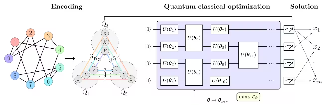In Abbildung 1 aus [1] wird des Max-Cut-Problem als Beispiel zur Veranschaulichung vom PCE-Ansatz verwendet. Des Max-Cut-Problem mit $m=9$ Knotn wird in an Pauli-Korrelationsraum kodiert, wobei des Optimierungsproblem als Korrelationsmatrix dargestellt wird, insbesondere als 2-Körper-Pauli-Matrix-Korrelationn über $n=3$ Qubits $(Q_1, Q_2, Q_3)$. Knotnfarbn gänd de Pauli-String aa, de für jedn kodiertn Knotn verwendet wird. Zum Beispiel wird Knotn 1, de de binärn Variabln $x_1$ entspricht, durch de Erwartungswert von $Z_1 \otimes Z_2 \otimes I_3$ kodiert, während $x_8$ durch $I_1 \otimes Y_2 \otimes Y_3$ kodiert wird. Des entspricht ra Kompression vo de $m$ Variabln vom Problem in $n = O(m^{1/2})$ Qubits. Allgemener ermöglichn $k$-Körper-Korrelationn polynomielle Kompressionen vo de Ordnung $k$. De gwählte Pauli-Satz umfasst drei Teilmengn vo gegaseitig kommutierenda Pauli-Strings, wodurch alle $m$ Korrelationn experimentell mit nur drei Messeinstellungen gschätzt wern könntn.

A Verlustfunktion $\mathcal{L}$ vo Pauli-Erwartungswerten, de de ursprüngliche Max-Cut-Zielfunktion nachahmt, wird konstruiert. De Verlustfunktion wird dann mit eim quante-klassischn Optimierungslöser wia dem Variational Quantum Eigensolver (VQE) optimiert.

Sobald de Optimierung abgschlossn is, wird de Lösung in de ursprüngliche Optimierungsraum zurückdekodiert, wodurch de optimale Max-Cut-Lösung erhoidn wird.

Aafordernisse

Stellts vor em Aafang vo dem Tutorial sicher, dass mia des Folgende installiert ham:

• Qiskit SDK v1.0 oder höher, mit Visualisierungs-Unterstützung
• Qiskit Runtime v0.22 oder höher (pip install qiskit-ibm-runtime)

Einrichtung

# Added by doQumentation — installs packages not in the Binder environment
!pip install -q networkx

from itertools import combinations

import numpy as np
import rustworkx as rx
from scipy.optimize import minimize

from qiskit.circuit.library import efficient_su2
from qiskit.transpiler.preset_passmanagers import generate_preset_pass_manager
from qiskit.quantum_info import SparsePauliOp
from qiskit_ibm_runtime import EstimatorV2 as Estimator
from qiskit_ibm_runtime import QiskitRuntimeService
from qiskit_ibm_runtime import Session
from rustworkx.visualization import mpl_draw

service = QiskitRuntimeService()
backend = service.least_busy(
    operational=True, simulator=False, min_num_qubits=127
)

def calc_cut_size(graph, partition0, partition1):
    """Calculate the cut size of the given partitions of the graph."""

    cut_size = 0
    for edge0, edge1 in graph.edge_list():
        if edge0 in partition0 and edge1 in partition1:
            cut_size += 1
        elif edge0 in partition1 and edge1 in partition0:
            cut_size += 1
    return cut_size

Schritt 1: Klassische Eingabn auf as Quanteproblem abbildn

Max-Cut-Problem

Des Max-Cut-Problem is a kombinatorisches Optimierungsproblem, des auf eim Graphen $G = (V, E)$ definiert is, wobei $V$ de Mengn vo de Knotn und $E$ de Mengn vo de Kantn is. Des Ziel is, de Knotn in zwoa Mengn $S$ und $V \setminus S$ z'partitioniern, sodass de Aazahl vo de Kantn zwischn de zwoa Mengn maximiert wird. Für a ausführliche Beschreibung vom Max-Cut-Problem verweists bitte auf des Tutorial "Quantum approximate optimization algorithm". Außerdem wird des Max-Cut-Problem als Beispiel im Tutorial "Advanced Techniques for QAOA" verwendet. In dene Tutorials wird de QAOA-Algorithmus zur Lösung vom Max-Cut-Problem eigsetzt.

Graph -> Hamiltonian

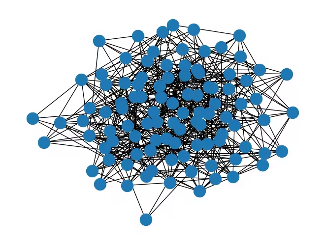
Des Tutorial verwendet an Zufallsgraphen mit 1000 Knotn.

De Problemgröße is möglicherweise schwer z'visualisiern, deshalb is untn a Graph mit 100 Knotn dargestellt. (De direkte Darstellung von eim Graphen mit 1.000 Knotn würd'n zu dicht mochn, um was z'segn!) De Graph, mit dem mia arbeitn, is zehnmal größer.

mpl_draw(rx.undirected_gnp_random_graph(100, 0.1, seed=42))

num_nodes = 1000  # Number of nodes in graph
graph = rx.undirected_gnp_random_graph(num_nodes, 0.1, seed=42)

import networkx as nx

nx_graph = nx.Graph()
nx_graph.add_nodes_from(range(num_nodes))

for edge in graph.edge_list():
    nx_graph.add_edge(edge[0], edge[1])

curr_cut_size, partition = nx.approximation.one_exchange(nx_graph, seed=1)
print(f"Initial cut size: {curr_cut_size}")

Initial cut size: 28075

Mia kodiern de Graphen mit 1000 Knotn in 2-Körper-Pauli-Matrix-Korrelationn über 100 Qubits. De Graph wird als Korrelationsmatrix dargestellt, wobei jeder Knotn durch an Pauli-String kodiert wird. Des Vorzeichen vom Erwartungswert vom Pauli-String gibt de Partition vom Knotn aa. Zum Beispiel wird Knotn 0 durch an Pauli-String kodiert, $\prod_0 = I_{19} \otimes ... I_2 \otimes X_1 \otimes X_0$. Des Vorzeichen vom Erwartungswert von dem Pauli-String gibt de Partition von Knotn 0 aa. Mia definieren a Pauli-Korrelations-Encoding (PCE) relativ zu $\prod$ als

$x_i \coloneqq \textit{sgn}(\langle\prod_i \rangle)$

wobei $x_i$ de Partition von Knotn $i$ is und $\langle \prod_i \rangle \coloneqq \langle \psi |\prod_i| \psi \rangle$ de Erwartungswert vom Pauli-String is, de Knotn $i$ über an Quantezustand $|\psi \rangle$ kodiert. Jetzt kodiern mia de Graphen mit PCE in an Hamiltonian. Mia teiln de Knotn in drei Mengn auf: $S_1$, $S_2$ und $S_3$. Dann kodiern mia de Knotn in jederer Mengn mit de Pauli-Strings $X$, $Y$ bzw. $Z$.

num_qubits = 100

list_size = num_nodes // 3
node_x = [i for i in range(list_size)]
node_y = [i for i in range(list_size, 2 * list_size)]
node_z = [i for i in range(2 * list_size, num_nodes)]

print("List 1:", node_x)
print("List 2:", node_y)
print("List 3:", node_z)

List 1: [0, 1, 2, 3, 4, 5, 6, 7, 8, 9, 10, 11, 12, 13, 14, 15, 16, 17, 18, 19, 20, 21, 22, 23, 24, 25, 26, 27, 28, 29, 30, 31, 32, 33, 34, 35, 36, 37, 38, 39, 40, 41, 42, 43, 44, 45, 46, 47, 48, 49, 50, 51, 52, 53, 54, 55, 56, 57, 58, 59, 60, 61, 62, 63, 64, 65, 66, 67, 68, 69, 70, 71, 72, 73, 74, 75, 76, 77, 78, 79, 80, 81, 82, 83, 84, 85, 86, 87, 88, 89, 90, 91, 92, 93, 94, 95, 96, 97, 98, 99, 100, 101, 102, 103, 104, 105, 106, 107, 108, 109, 110, 111, 112, 113, 114, 115, 116, 117, 118, 119, 120, 121, 122, 123, 124, 125, 126, 127, 128, 129, 130, 131, 132, 133, 134, 135, 136, 137, 138, 139, 140, 141, 142, 143, 144, 145, 146, 147, 148, 149, 150, 151, 152, 153, 154, 155, 156, 157, 158, 159, 160, 161, 162, 163, 164, 165, 166, 167, 168, 169, 170, 171, 172, 173, 174, 175, 176, 177, 178, 179, 180, 181, 182, 183, 184, 185, 186, 187, 188, 189, 190, 191, 192, 193, 194, 195, 196, 197, 198, 199, 200, 201, 202, 203, 204, 205, 206, 207, 208, 209, 210, 211, 212, 213, 214, 215, 216, 217, 218, 219, 220, 221, 222, 223, 224, 225, 226, 227, 228, 229, 230, 231, 232, 233, 234, 235, 236, 237, 238, 239, 240, 241, 242, 243, 244, 245, 246, 247, 248, 249, 250, 251, 252, 253, 254, 255, 256, 257, 258, 259, 260, 261, 262, 263, 264, 265, 266, 267, 268, 269, 270, 271, 272, 273, 274, 275, 276, 277, 278, 279, 280, 281, 282, 283, 284, 285, 286, 287, 288, 289, 290, 291, 292, 293, 294, 295, 296, 297, 298, 299, 300, 301, 302, 303, 304, 305, 306, 307, 308, 309, 310, 311, 312, 313, 314, 315, 316, 317, 318, 319, 320, 321, 322, 323, 324, 325, 326, 327, 328, 329, 330, 331, 332]
List 2: [333, 334, 335, 336, 337, 338, 339, 340, 341, 342, 343, 344, 345, 346, 347, 348, 349, 350, 351, 352, 353, 354, 355, 356, 357, 358, 359, 360, 361, 362, 363, 364, 365, 366, 367, 368, 369, 370, 371, 372, 373, 374, 375, 376, 377, 378, 379, 380, 381, 382, 383, 384, 385, 386, 387, 388, 389, 390, 391, 392, 393, 394, 395, 396, 397, 398, 399, 400, 401, 402, 403, 404, 405, 406, 407, 408, 409, 410, 411, 412, 413, 414, 415, 416, 417, 418, 419, 420, 421, 422, 423, 424, 425, 426, 427, 428, 429, 430, 431, 432, 433, 434, 435, 436, 437, 438, 439, 440, 441, 442, 443, 444, 445, 446, 447, 448, 449, 450, 451, 452, 453, 454, 455, 456, 457, 458, 459, 460, 461, 462, 463, 464, 465, 466, 467, 468, 469, 470, 471, 472, 473, 474, 475, 476, 477, 478, 479, 480, 481, 482, 483, 484, 485, 486, 487, 488, 489, 490, 491, 492, 493, 494, 495, 496, 497, 498, 499, 500, 501, 502, 503, 504, 505, 506, 507, 508, 509, 510, 511, 512, 513, 514, 515, 516, 517, 518, 519, 520, 521, 522, 523, 524, 525, 526, 527, 528, 529, 530, 531, 532, 533, 534, 535, 536, 537, 538, 539, 540, 541, 542, 543, 544, 545, 546, 547, 548, 549, 550, 551, 552, 553, 554, 555, 556, 557, 558, 559, 560, 561, 562, 563, 564, 565, 566, 567, 568, 569, 570, 571, 572, 573, 574, 575, 576, 577, 578, 579, 580, 581, 582, 583, 584, 585, 586, 587, 588, 589, 590, 591, 592, 593, 594, 595, 596, 597, 598, 599, 600, 601, 602, 603, 604, 605, 606, 607, 608, 609, 610, 611, 612, 613, 614, 615, 616, 617, 618, 619, 620, 621, 622, 623, 624, 625, 626, 627, 628, 629, 630, 631, 632, 633, 634, 635, 636, 637, 638, 639, 640, 641, 642, 643, 644, 645, 646, 647, 648, 649, 650, 651, 652, 653, 654, 655, 656, 657, 658, 659, 660, 661, 662, 663, 664, 665]
List 3: [666, 667, 668, 669, 670, 671, 672, 673, 674, 675, 676, 677, 678, 679, 680, 681, 682, 683, 684, 685, 686, 687, 688, 689, 690, 691, 692, 693, 694, 695, 696, 697, 698, 699, 700, 701, 702, 703, 704, 705, 706, 707, 708, 709, 710, 711, 712, 713, 714, 715, 716, 717, 718, 719, 720, 721, 722, 723, 724, 725, 726, 727, 728, 729, 730, 731, 732, 733, 734, 735, 736, 737, 738, 739, 740, 741, 742, 743, 744, 745, 746, 747, 748, 749, 750, 751, 752, 753, 754, 755, 756, 757, 758, 759, 760, 761, 762, 763, 764, 765, 766, 767, 768, 769, 770, 771, 772, 773, 774, 775, 776, 777, 778, 779, 780, 781, 782, 783, 784, 785, 786, 787, 788, 789, 790, 791, 792, 793, 794, 795, 796, 797, 798, 799, 800, 801, 802, 803, 804, 805, 806, 807, 808, 809, 810, 811, 812, 813, 814, 815, 816, 817, 818, 819, 820, 821, 822, 823, 824, 825, 826, 827, 828, 829, 830, 831, 832, 833, 834, 835, 836, 837, 838, 839, 840, 841, 842, 843, 844, 845, 846, 847, 848, 849, 850, 851, 852, 853, 854, 855, 856, 857, 858, 859, 860, 861, 862, 863, 864, 865, 866, 867, 868, 869, 870, 871, 872, 873, 874, 875, 876, 877, 878, 879, 880, 881, 882, 883, 884, 885, 886, 887, 888, 889, 890, 891, 892, 893, 894, 895, 896, 897, 898, 899, 900, 901, 902, 903, 904, 905, 906, 907, 908, 909, 910, 911, 912, 913, 914, 915, 916, 917, 918, 919, 920, 921, 922, 923, 924, 925, 926, 927, 928, 929, 930, 931, 932, 933, 934, 935, 936, 937, 938, 939, 940, 941, 942, 943, 944, 945, 946, 947, 948, 949, 950, 951, 952, 953, 954, 955, 956, 957, 958, 959, 960, 961, 962, 963, 964, 965, 966, 967, 968, 969, 970, 971, 972, 973, 974, 975, 976, 977, 978, 979, 980, 981, 982, 983, 984, 985, 986, 987, 988, 989, 990, 991, 992, 993, 994, 995, 996, 997, 998, 999]

def build_pauli_correlation_encoding(pauli, node_list, n, k=2):
    pauli_correlation_encoding = []
    for idx, c in enumerate(combinations(range(n), k)):
        if idx >= len(node_list):
            break
        paulis = ["I"] * n
        paulis[c[0]], paulis[c[1]] = pauli, pauli
        pauli_correlation_encoding.append(("".join(paulis)[::-1], 1))

    hamiltonian = []
    for pauli, weight in pauli_correlation_encoding:
        hamiltonian.append(SparsePauliOp.from_list([(pauli, weight)]))

    return hamiltonian

pauli_correlation_encoding_x = build_pauli_correlation_encoding(
    "X", node_x, num_qubits
)
pauli_correlation_encoding_y = build_pauli_correlation_encoding(
    "Y", node_y, num_qubits
)
pauli_correlation_encoding_z = build_pauli_correlation_encoding(
    "Z", node_z, num_qubits
)

Schritt 2: Problem für de Ausführung auf Quante-Hardware optimiern

Quanteschaltkreis

Do wird de Zustand $|\psi \rangle$ mit $\mathbf{\theta}$ parametrisiert, und mia optimiern dene Parameter $\mathbf{\theta}$ mit eim variationelln Ansatz. Des Tutorial verwendet de efficient_su2 Ansatz für unsern variationelln Algorithmus wegen seiner Ausdrucksfähigkeit und einfachn Implementierung. Mia verwendn aa de relaxierte Verlustfunktion, de später in dem Tutorial eigführt wird. Als Ergebnis kennma großskalige Probleme mit weniger Qubits und geringern Schaltkreistiefen aagehen.

# Build the quantum circuit
qc = efficient_su2(num_qubits, ["ry", "rz"], reps=2)

# Optimize the circuit

pm = generate_preset_pass_manager(optimization_level=3, backend=backend)
qc = pm.run(qc)

Verlustfunktion

Für de Verlustfunktion $\mathcal{L}$ verwendn mia a Relaxation vo de Max-Cut-Zielfunktion wia in [1] beschrieben, de als $\mathcal{V}(\mathbf{x}) \coloneqq \sum_{(i, j) \in E} W_{i, j}(1-x_i x_j)$ definiert is. Do bezeichnet $W_{i, j}$ des Gwicht vo de Kante $(i, j)$ und $x_i$ de Partition von Knotn $i$. De Verlustfunktion $\mathcal{L}$ is gegeben durch:

$\mathcal{L}\coloneqq \sum_{(i, j) \in E} W_{i, j} \text{tanh} (\alpha \langle\prod_i \rangle) \text{tanh} (\alpha \langle\prod_j \rangle) + \mathcal{L}^{(\text{reg})}$

wobei de Max-Cut-Zielfunktion durch glatte hyperbolische Tangenten vo de Erwartungswerten vo de Pauli-Strings ersetzt wird, de de Knotn kodiern. De Regularisierungsterm $\mathcal{L}^{(\text{reg})}$ und de Skalierungsfaktor $\alpha$, proportional zur Aazahl vo de Qubits, wern eigführt, um de Leistung vom Löser z'verbessern.

De Regularisierungsterm is definiert als:

$\mathcal{L}^{(\text{reg})}$ is definiert als $\mathcal{L}^{(\text{reg})} \coloneqq \beta \nu \lbrack \frac{1}{m} \sum_{i \in V} \text{tanh} (\alpha \langle\prod_i \rangle)^2 \rbrack ^2$

wobei $\beta=1/2$, $\nu = |E|/2 + (m -1) /4$ und $m$ de Aazahl vo de Knotn im Graphen is.

def loss_func_estimator(x, ansatz, hamiltonian, estimator, graph):
    """
    Calculates the specified loss function for the given ansatz, Hamiltonian, and graph.

    The expectation values of each Pauli string in the Hamiltonian are first obtained
    by running the ansatz on the quantum backend. These expectation values are then
    passed through the nonlinear function tanh(alpha * prod_i). The loss function is
    subsequently computed from these transformed values.
    """
    job = estimator.run(
        [
            (ansatz, hamiltonian[0], x),
            (ansatz, hamiltonian[1], x),
            (ansatz, hamiltonian[2], x),
        ]
    )
    result = job.result()

    # calculate the loss function
    node_exp_map = {}
    idx = 0
    for r in result:
        for ev in r.data.evs:
            node_exp_map[idx] = ev
            idx += 1

    loss = 0
    alpha = num_qubits
    for edge0, edge1 in graph.edge_list():
        loss += np.tanh(alpha * node_exp_map[edge0]) * np.tanh(
            alpha * node_exp_map[edge1]
        )

    regulation_term = 0
    for i in range(len(graph.nodes())):
        regulation_term += np.tanh(alpha * node_exp_map[i]) ** 2
    regulation_term = regulation_term / len(graph.nodes())
    regulation_term = regulation_term**2
    beta = 1 / 2
    v = len(graph.edges()) / 2 + (len(graph.nodes()) - 1) / 4
    regulation_term = beta * v * regulation_term

    loss = loss + regulation_term

    global experiment_result
    print(f"Iter {len(experiment_result)}: {loss}")
    experiment_result.append({"loss": loss, "exp_map": node_exp_map})
    return loss

Schritt 3: Ausführung mit Qiskit Primitives

In dem Tutorial setzen mia max_iter=50 für de Optimierungsschleife zu Demonstrationszwecken. Wenn mia de Aazahl vo de Iterationn erhöhen, kenna mia bessere Ergebnisse erwarten.

pce = []
pce.append(
    [op.apply_layout(qc.layout) for op in pauli_correlation_encoding_x]
)
pce.append(
    [op.apply_layout(qc.layout) for op in pauli_correlation_encoding_y]
)
pce.append(
    [op.apply_layout(qc.layout) for op in pauli_correlation_encoding_z]
)

# Run the optimization using Session

with Session(backend=backend) as session:
    estimator = Estimator(mode=session)

    experiment_result = []

    def loss_func(x):
        return loss_func_estimator(
            x, qc, [pce[0], pce[1], pce[2]], estimator, graph
        )

    np.random.seed(42)
    initial_params = np.random.rand(qc.num_parameters)
    result = minimize(
        loss_func, initial_params, method="COBYLA", options={"maxiter": 50}
    )
print(result)

Iter 0: 16659.649201600296
Iter 1: 12104.242957555361
Iter 2: 6541.137221994661
Iter 3: 6650.6188244671985
Iter 4: 7033.193518185085
Iter 5: 6743.687931793412
Iter 6: 6223.574718684094
Iter 7: 6457.3302709535965
Iter 8: 6581.316449107595
Iter 9: 6365.761052029896
Iter 10: 6415.872673527322
Iter 11: 6421.996561600348
Iter 12: 6636.372822791712
Iter 13: 6965.174320702346
Iter 14: 6774.236562696287
Iter 15: 6393.837617108355
Iter 16: 6234.311401676519
Iter 17: 6518.192237615901
Iter 18: 6559.933925068997
Iter 19: 6646.157979243488
Iter 20: 6573.726111605048
Iter 21: 6190.642092901959
Iter 22: 6653.06500163594
Iter 23: 6545.713700369988
Iter 24: 6399.996441760465
Iter 25: 6115.959687941808
Iter 26: 6665.915093554849
Iter 27: 6832.882201259893
Iter 28: 6541.392749578919
Iter 29: 6813.3456910443165
Iter 30: 6460.800944368402
Iter 31: 6359.635437029245
Iter 32: 6040.891641882451
Iter 33: 6573.930674936448
Iter 34: 6668.031753293785
Iter 35: 6450.002712889748
Iter 36: 6519.8298811058075
Iter 37: 6467.134502398199
Iter 38: 6655.284651397334
Iter 39: 6371.168353987336
Iter 40: 6480.337259347923
Iter 41: 6339.256786764425
Iter 42: 6588.635046825541
Iter 43: 6617.677964971322
Iter 44: 6469.0441600679205
Iter 45: 6567.874244906106
Iter 46: 6217.899975264532
Iter 47: 6783.481394627947
Iter 48: 6813.371853626112
Iter 49: 6506.5871531488765
 message: Maximum number of function evaluations has been exceeded.
 success: False
  status: 2
     fun: 6040.891641882451
       x: [ 1.375e+00  1.951e+00 ...  1.923e-01  4.087e-02]
    nfev: 50
   maxcv: 0.0

Schritt 4: Nachbearbeitung und Rückgabe vom Ergebnis im gwünschtn klassischn Format

De Partitionn vo de Knotn wern durch Auswertung vom Vorzeichen vo de Erwartungswerten vo de Pauli-Strings bestimmt, de de Knotn kodiern.

# Calculate the partitions based on the final expectation values
# If the expectation value is positive, the node belongs to partition 0 (par0)
# Otherwise, the node belongs to partition 1 (par1)

par0, par1 = set(), set()

for i in experiment_result[-1]["exp_map"]:
    if experiment_result[-1]["exp_map"][i] >= 0:
        par0.add(i)
    else:
        par1.add(i)
print(par0, par1)

{0, 1, 4, 8, 9, 10, 12, 13, 14, 15, 16, 18, 25, 27, 31, 32, 34, 36, 38, 39, 40, 41, 44, 46, 47, 48, 49, 50, 51, 52, 57, 60, 61, 62, 63, 64, 65, 66, 68, 71, 79, 81, 82, 86, 88, 91, 92, 93, 94, 95, 96, 99, 100, 105, 106, 107, 112, 114, 115, 121, 123, 129, 133, 134, 145, 147, 161, 165, 166, 168, 171, 173, 184, 185, 187, 188, 192, 193, 194, 196, 197, 198, 202, 205, 206, 207, 208, 209, 210, 211, 215, 217, 218, 219, 220, 221, 225, 226, 227, 228, 229, 230, 231, 232, 233, 234, 235, 236, 238, 241, 242, 243, 244, 246, 247, 248, 249, 251, 252, 253, 255, 256, 257, 258, 259, 261, 262, 264, 265, 266, 268, 269, 270, 272, 273, 275, 276, 277, 278, 279, 281, 283, 284, 285, 286, 288, 292, 293, 294, 299, 300, 303, 305, 306, 307, 308, 310, 312, 313, 314, 316, 317, 319, 321, 326, 327, 328, 333, 336, 338, 340, 341, 342, 344, 345, 346, 349, 351, 352, 353, 356, 357, 360, 361, 362, 363, 364, 366, 368, 370, 374, 378, 379, 380, 381, 382, 383, 384, 386, 387, 388, 389, 390, 391, 393, 394, 395, 396, 397, 398, 404, 405, 406, 409, 411, 413, 415, 416, 418, 421, 425, 426, 427, 428, 429, 433, 434, 435, 437, 444, 450, 456, 457, 458, 459, 462, 463, 465, 467, 469, 470, 472, 476, 479, 484, 487, 489, 492, 493, 497, 498, 499, 502, 506, 508, 513, 516, 517, 518, 519, 521, 523, 526, 527, 528, 531, 532, 533, 535, 536, 537, 539, 540, 541, 542, 543, 544, 545, 547, 549, 550, 552, 557, 562, 563, 564, 565, 567, 568, 569, 570, 571, 572, 573, 576, 578, 579, 580, 583, 585, 587, 588, 589, 591, 595, 596, 597, 600, 602, 603, 604, 605, 606, 607, 608, 609, 610, 612, 618, 619, 623, 624, 625, 626, 627, 628, 630, 632, 636, 637, 640, 644, 646, 649, 652, 656, 657, 658, 659, 661, 662, 663, 664, 667, 669, 670, 671, 672, 674, 675, 676, 677, 678, 679, 680, 681, 682, 683, 684, 685, 686, 687, 688, 689, 690, 692, 693, 694, 695, 696, 698, 700, 701, 703, 706, 707, 708, 709, 712, 713, 714, 716, 717, 718, 719, 721, 722, 723, 724, 725, 726, 728, 730, 731, 733, 734, 735, 737, 739, 740, 741, 743, 744, 746, 748, 750, 751, 752, 753, 754, 758, 760, 761, 762, 763, 764, 765, 766, 774, 778, 780, 782, 787, 795, 800, 802, 803, 808, 809, 812, 818, 822, 825, 827, 834, 836, 840, 843, 845, 847, 850, 853, 854, 857, 858, 863, 864, 865, 866, 867, 868, 869, 870, 872, 873, 874, 875, 876, 878, 880, 881, 882, 883, 884, 885, 887, 888, 889, 890, 891, 893, 894, 895, 896, 898, 901, 902, 903, 904, 905, 907, 908, 910, 911, 912, 913, 914, 915, 916, 917, 918, 920, 921, 923, 925, 926, 928, 929, 930, 932, 934, 935, 936, 938, 939, 941, 943, 945, 946, 947, 948, 949, 953, 955, 956, 957, 958, 959, 961, 966, 975, 978, 980, 983, 988, 990, 996, 999} {2, 3, 5, 6, 7, 11, 17, 19, 20, 21, 22, 23, 24, 26, 28, 29, 30, 33, 35, 37, 42, 43, 45, 53, 54, 55, 56, 58, 59, 67, 69, 70, 72, 73, 74, 75, 76, 77, 78, 80, 83, 84, 85, 87, 89, 90, 97, 98, 101, 102, 103, 104, 108, 109, 110, 111, 113, 116, 117, 118, 119, 120, 122, 124, 125, 126, 127, 128, 130, 131, 132, 135, 136, 137, 138, 139, 140, 141, 142, 143, 144, 146, 148, 149, 150, 151, 152, 153, 154, 155, 156, 157, 158, 159, 160, 162, 163, 164, 167, 169, 170, 172, 174, 175, 176, 177, 178, 179, 180, 181, 182, 183, 186, 189, 190, 191, 195, 199, 200, 201, 203, 204, 212, 213, 214, 216, 222, 223, 224, 237, 239, 240, 245, 250, 254, 260, 263, 267, 271, 274, 280, 282, 287, 289, 290, 291, 295, 296, 297, 298, 301, 302, 304, 309, 311, 315, 318, 320, 322, 323, 324, 325, 329, 330, 331, 332, 334, 335, 337, 339, 343, 347, 348, 350, 354, 355, 358, 359, 365, 367, 369, 371, 372, 373, 375, 376, 377, 385, 392, 399, 400, 401, 402, 403, 407, 408, 410, 412, 414, 417, 419, 420, 422, 423, 424, 430, 431, 432, 436, 438, 439, 440, 441, 442, 443, 445, 446, 447, 448, 449, 451, 452, 453, 454, 455, 460, 461, 464, 466, 468, 471, 473, 474, 475, 477, 478, 480, 481, 482, 483, 485, 486, 488, 490, 491, 494, 495, 496, 500, 501, 503, 504, 505, 507, 509, 510, 511, 512, 514, 515, 520, 522, 524, 525, 529, 530, 534, 538, 546, 548, 551, 553, 554, 555, 556, 558, 559, 560, 561, 566, 574, 575, 577, 581, 582, 584, 586, 590, 592, 593, 594, 598, 599, 601, 611, 613, 614, 615, 616, 617, 620, 621, 622, 629, 631, 633, 634, 635, 638, 639, 641, 642, 643, 645, 647, 648, 650, 651, 653, 654, 655, 660, 665, 666, 668, 673, 691, 697, 699, 702, 704, 705, 710, 711, 715, 720, 727, 729, 732, 736, 738, 742, 745, 747, 749, 755, 756, 757, 759, 767, 768, 769, 770, 771, 772, 773, 775, 776, 777, 779, 781, 783, 784, 785, 786, 788, 789, 790, 791, 792, 793, 794, 796, 797, 798, 799, 801, 804, 805, 806, 807, 810, 811, 813, 814, 815, 816, 817, 819, 820, 821, 823, 824, 826, 828, 829, 830, 831, 832, 833, 835, 837, 838, 839, 841, 842, 844, 846, 848, 849, 851, 852, 855, 856, 859, 860, 861, 862, 871, 877, 879, 886, 892, 897, 899, 900, 906, 909, 919, 922, 924, 927, 931, 933, 937, 940, 942, 944, 950, 951, 952, 954, 960, 962, 963, 964, 965, 967, 968, 969, 970, 971, 972, 973, 974, 976, 977, 979, 981, 982, 984, 985, 986, 987, 989, 991, 992, 993, 994, 995, 997, 998}

Mia kenna de Cut-Größe vom Max-Cut-Problem mit de Partitionn vo de Knotn berechnen.

cut_size = calc_cut_size(graph, par0, par1)
print(f"Cut size: {cut_size}")

Cut size: 24682

Sobald des Training abgschlossn is, führn mia a Runde Single-Bit-Swap-Suche durch, um de Lösung als klassischn Nachbearbeitungsschritt z'verbessern. Bei dem Prozess tauschen mia de Partitionn von zwoa Knotn und bewerten de Cut-Größe. Wenn de Cut-Größe verbessert wird, bhaltn mia de Tausch. Mia wiederholn dene Prozess für alle möglichn Knotenpaare, de durch a Kante verbundn san.

best_bits = []
cur_bits = []

for i in experiment_result[-1]["exp_map"]:
    if experiment_result[-1]["exp_map"][i] >= 0:
        cur_bits.append(1)
    else:
        cur_bits.append(0)
print(cur_bits)

[1, 1, 0, 0, 1, 0, 0, 0, 1, 1, 1, 0, 1, 1, 1, 1, 1, 0, 1, 0, 0, 0, 0, 0, 0, 1, 0, 1, 0, 0, 0, 1, 1, 0, 1, 0, 1, 0, 1, 1, 1, 1, 0, 0, 1, 0, 1, 1, 1, 1, 1, 1, 1, 0, 0, 0, 0, 1, 0, 0, 1, 1, 1, 1, 1, 1, 1, 0, 1, 0, 0, 1, 0, 0, 0, 0, 0, 0, 0, 1, 0, 1, 1, 0, 0, 0, 1, 0, 1, 0, 0, 1, 1, 1, 1, 1, 1, 0, 0, 1, 1, 0, 0, 0, 0, 1, 1, 1, 0, 0, 0, 0, 1, 0, 1, 1, 0, 0, 0, 0, 0, 1, 0, 1, 0, 0, 0, 0, 0, 1, 0, 0, 0, 1, 1, 0, 0, 0, 0, 0, 0, 0, 0, 0, 0, 1, 0, 1, 0, 0, 0, 0, 0, 0, 0, 0, 0, 0, 0, 0, 0, 1, 0, 0, 0, 1, 1, 0, 1, 0, 0, 1, 0, 1, 0, 0, 0, 0, 0, 0, 0, 0, 0, 0, 1, 1, 0, 1, 1, 0, 0, 0, 1, 1, 1, 0, 1, 1, 1, 0, 0, 0, 1, 0, 0, 1, 1, 1, 1, 1, 1, 1, 0, 0, 0, 1, 0, 1, 1, 1, 1, 1, 0, 0, 0, 1, 1, 1, 1, 1, 1, 1, 1, 1, 1, 1, 1, 0, 1, 0, 0, 1, 1, 1, 1, 0, 1, 1, 1, 1, 0, 1, 1, 1, 0, 1, 1, 1, 1, 1, 0, 1, 1, 0, 1, 1, 1, 0, 1, 1, 1, 0, 1, 1, 0, 1, 1, 1, 1, 1, 0, 1, 0, 1, 1, 1, 1, 0, 1, 0, 0, 0, 1, 1, 1, 0, 0, 0, 0, 1, 1, 0, 0, 1, 0, 1, 1, 1, 1, 0, 1, 0, 1, 1, 1, 0, 1, 1, 0, 1, 0, 1, 0, 0, 0, 0, 1, 1, 1, 0, 0, 0, 0, 1, 0, 0, 1, 0, 1, 0, 1, 1, 1, 0, 1, 1, 1, 0, 0, 1, 0, 1, 1, 1, 0, 0, 1, 1, 0, 0, 1, 1, 1, 1, 1, 0, 1, 0, 1, 0, 1, 0, 0, 0, 1, 0, 0, 0, 1, 1, 1, 1, 1, 1, 1, 0, 1, 1, 1, 1, 1, 1, 0, 1, 1, 1, 1, 1, 1, 0, 0, 0, 0, 0, 1, 1, 1, 0, 0, 1, 0, 1, 0, 1, 0, 1, 1, 0, 1, 0, 0, 1, 0, 0, 0, 1, 1, 1, 1, 1, 0, 0, 0, 1, 1, 1, 0, 1, 0, 0, 0, 0, 0, 0, 1, 0, 0, 0, 0, 0, 1, 0, 0, 0, 0, 0, 1, 1, 1, 1, 0, 0, 1, 1, 0, 1, 0, 1, 0, 1, 1, 0, 1, 0, 0, 0, 1, 0, 0, 1, 0, 0, 0, 0, 1, 0, 0, 1, 0, 1, 0, 0, 1, 1, 0, 0, 0, 1, 1, 1, 0, 0, 1, 0, 0, 0, 1, 0, 1, 0, 0, 0, 0, 1, 0, 0, 1, 1, 1, 1, 0, 1, 0, 1, 0, 0, 1, 1, 1, 0, 0, 1, 1, 1, 0, 1, 1, 1, 0, 1, 1, 1, 1, 1, 1, 1, 0, 1, 0, 1, 1, 0, 1, 0, 0, 0, 0, 1, 0, 0, 0, 0, 1, 1, 1, 1, 0, 1, 1, 1, 1, 1, 1, 1, 0, 0, 1, 0, 1, 1, 1, 0, 0, 1, 0, 1, 0, 1, 1, 1, 0, 1, 0, 0, 0, 1, 1, 1, 0, 0, 1, 0, 1, 1, 1, 1, 1, 1, 1, 1, 1, 0, 1, 0, 0, 0, 0, 0, 1, 1, 0, 0, 0, 1, 1, 1, 1, 1, 1, 0, 1, 0, 1, 0, 0, 0, 1, 1, 0, 0, 1, 0, 0, 0, 1, 0, 1, 0, 0, 1, 0, 0, 1, 0, 0, 0, 1, 1, 1, 1, 0, 1, 1, 1, 1, 0, 0, 1, 0, 1, 1, 1, 1, 0, 1, 1, 1, 1, 1, 1, 1, 1, 1, 1, 1, 1, 1, 1, 1, 1, 1, 0, 1, 1, 1, 1, 1, 0, 1, 0, 1, 1, 0, 1, 0, 0, 1, 1, 1, 1, 0, 0, 1, 1, 1, 0, 1, 1, 1, 1, 0, 1, 1, 1, 1, 1, 1, 0, 1, 0, 1, 1, 0, 1, 1, 1, 0, 1, 0, 1, 1, 1, 0, 1, 1, 0, 1, 0, 1, 0, 1, 1, 1, 1, 1, 0, 0, 0, 1, 0, 1, 1, 1, 1, 1, 1, 1, 0, 0, 0, 0, 0, 0, 0, 1, 0, 0, 0, 1, 0, 1, 0, 1, 0, 0, 0, 0, 1, 0, 0, 0, 0, 0, 0, 0, 1, 0, 0, 0, 0, 1, 0, 1, 1, 0, 0, 0, 0, 1, 1, 0, 0, 1, 0, 0, 0, 0, 0, 1, 0, 0, 0, 1, 0, 0, 1, 0, 1, 0, 0, 0, 0, 0, 0, 1, 0, 1, 0, 0, 0, 1, 0, 0, 1, 0, 1, 0, 1, 0, 0, 1, 0, 0, 1, 1, 0, 0, 1, 1, 0, 0, 0, 0, 1, 1, 1, 1, 1, 1, 1, 1, 0, 1, 1, 1, 1, 1, 0, 1, 0, 1, 1, 1, 1, 1, 1, 0, 1, 1, 1, 1, 1, 0, 1, 1, 1, 1, 0, 1, 0, 0, 1, 1, 1, 1, 1, 0, 1, 1, 0, 1, 1, 1, 1, 1, 1, 1, 1, 1, 0, 1, 1, 0, 1, 0, 1, 1, 0, 1, 1, 1, 0, 1, 0, 1, 1, 1, 0, 1, 1, 0, 1, 0, 1, 0, 1, 1, 1, 1, 1, 0, 0, 0, 1, 0, 1, 1, 1, 1, 1, 0, 1, 0, 0, 0, 0, 1, 0, 0, 0, 0, 0, 0, 0, 0, 1, 0, 0, 1, 0, 1, 0, 0, 1, 0, 0, 0, 0, 1, 0, 1, 0, 0, 0, 0, 0, 1, 0, 0, 1]

# Swap the partitions and calculate the cut size
best_cut = 0
for edge0, edge1 in graph.edge_list():
    swapped_bits = cur_bits.copy()
    swapped_bits[edge0], swapped_bits[edge1] = (
        swapped_bits[edge1],
        swapped_bits[edge0],
    )

    cur_partition = [set(), set()]
    for i, bit in enumerate(swapped_bits):
        if bit > 0:
            cur_partition[0].add(i)
        else:
            cur_partition[1].add(i)
    cut_size = calc_cut_size(graph, cur_partition[0], cur_partition[1])
    if best_cut < cut_size:
        best_cut = cut_size
        best_bits = swapped_bits

print(best_cut, best_bits)

24733 [1, 1, 0, 0, 1, 0, 0, 0, 1, 1, 1, 0, 1, 1, 1, 1, 1, 0, 1, 0, 0, 0, 0, 0, 0, 1, 0, 1, 0, 0, 0, 1, 1, 0, 1, 0, 1, 0, 1, 1, 1, 1, 0, 0, 1, 0, 1, 1, 1, 1, 1, 1, 1, 0, 0, 0, 0, 1, 0, 0, 1, 1, 1, 1, 1, 1, 1, 0, 1, 0, 0, 1, 0, 0, 0, 0, 0, 0, 0, 1, 0, 1, 1, 0, 0, 0, 1, 0, 1, 0, 0, 1, 1, 1, 1, 1, 1, 0, 0, 1, 1, 0, 0, 0, 0, 1, 1, 1, 0, 0, 0, 0, 1, 0, 1, 1, 0, 0, 0, 0, 0, 1, 0, 1, 0, 0, 0, 0, 0, 1, 0, 0, 0, 1, 1, 0, 0, 0, 0, 0, 0, 0, 0, 0, 0, 1, 0, 1, 0, 0, 0, 0, 0, 0, 0, 0, 0, 0, 0, 0, 0, 1, 0, 0, 0, 1, 1, 0, 1, 0, 0, 1, 0, 1, 0, 0, 0, 0, 0, 0, 0, 0, 0, 0, 1, 1, 0, 1, 1, 0, 0, 0, 1, 1, 1, 0, 1, 1, 1, 0, 0, 0, 1, 0, 0, 1, 1, 1, 1, 1, 1, 1, 0, 0, 0, 1, 0, 1, 1, 1, 1, 1, 0, 0, 0, 1, 1, 1, 1, 1, 1, 1, 1, 1, 1, 1, 1, 0, 1, 0, 0, 1, 1, 1, 1, 0, 0, 1, 1, 1, 0, 1, 1, 1, 0, 1, 1, 1, 1, 1, 0, 1, 1, 0, 1, 1, 1, 0, 1, 1, 1, 0, 1, 1, 0, 1, 1, 1, 1, 1, 0, 1, 0, 1, 1, 1, 1, 0, 1, 0, 0, 0, 1, 1, 1, 0, 0, 0, 0, 1, 1, 0, 0, 1, 0, 1, 1, 1, 1, 0, 1, 0, 1, 1, 1, 0, 1, 1, 0, 1, 0, 1, 0, 0, 0, 0, 1, 1, 1, 0, 0, 0, 0, 1, 0, 0, 1, 0, 1, 0, 1, 1, 1, 0, 1, 1, 1, 0, 0, 1, 0, 1, 1, 1, 0, 0, 1, 1, 0, 0, 1, 1, 1, 1, 1, 0, 1, 0, 1, 0, 1, 0, 0, 0, 1, 0, 0, 0, 1, 1, 1, 1, 1, 1, 1, 0, 1, 1, 1, 1, 1, 1, 0, 1, 1, 1, 1, 1, 1, 0, 0, 0, 0, 0, 1, 1, 1, 0, 0, 1, 0, 1, 0, 1, 0, 1, 1, 0, 1, 0, 0, 1, 0, 0, 0, 1, 1, 1, 1, 1, 0, 0, 0, 1, 1, 1, 0, 1, 0, 0, 0, 0, 0, 0, 1, 0, 0, 0, 0, 0, 1, 0, 0, 0, 0, 0, 1, 1, 1, 1, 0, 0, 1, 1, 0, 1, 0, 1, 0, 1, 1, 0, 1, 0, 0, 0, 1, 0, 0, 1, 0, 0, 0, 0, 1, 0, 0, 1, 0, 1, 0, 0, 1, 1, 0, 0, 0, 1, 1, 1, 0, 0, 1, 0, 0, 0, 1, 0, 1, 0, 0, 0, 0, 1, 0, 0, 1, 1, 1, 1, 0, 1, 0, 1, 0, 0, 1, 1, 1, 0, 0, 1, 1, 1, 0, 1, 1, 1, 0, 1, 1, 1, 1, 1, 1, 1, 0, 1, 0, 1, 1, 0, 1, 0, 0, 0, 0, 1, 0, 0, 0, 0, 1, 1, 1, 1, 0, 1, 1, 1, 1, 1, 1, 1, 0, 0, 1, 0, 1, 1, 1, 0, 0, 1, 0, 1, 0, 1, 1, 1, 0, 1, 0, 0, 0, 1, 1, 1, 0, 0, 1, 0, 1, 1, 1, 1, 1, 1, 1, 1, 1, 0, 1, 0, 0, 0, 0, 0, 1, 1, 0, 0, 0, 1, 1, 1, 1, 1, 1, 0, 1, 0, 1, 0, 1, 0, 1, 1, 0, 0, 1, 0, 0, 0, 1, 0, 1, 0, 0, 1, 0, 0, 1, 0, 0, 0, 1, 1, 1, 1, 0, 1, 1, 1, 1, 0, 0, 1, 0, 1, 1, 1, 1, 0, 1, 1, 1, 1, 1, 1, 1, 1, 1, 1, 1, 1, 1, 1, 1, 1, 1, 0, 1, 1, 1, 1, 1, 0, 1, 0, 1, 1, 0, 1, 0, 0, 1, 1, 1, 1, 0, 0, 1, 1, 1, 0, 1, 1, 1, 1, 0, 1, 1, 1, 1, 1, 1, 0, 1, 0, 1, 1, 0, 1, 1, 1, 0, 1, 0, 1, 1, 1, 0, 1, 1, 0, 1, 0, 1, 0, 1, 1, 1, 1, 1, 0, 0, 0, 1, 0, 1, 1, 1, 1, 1, 1, 1, 0, 0, 0, 0, 0, 0, 0, 1, 0, 0, 0, 1, 0, 1, 0, 1, 0, 0, 0, 0, 1, 0, 0, 0, 0, 0, 0, 0, 1, 0, 0, 0, 0, 1, 0, 1, 1, 0, 0, 0, 0, 1, 1, 0, 0, 1, 0, 0, 0, 0, 0, 1, 0, 0, 0, 1, 0, 0, 1, 0, 1, 0, 0, 0, 0, 0, 0, 1, 0, 1, 0, 0, 0, 1, 0, 0, 1, 0, 1, 0, 1, 0, 0, 1, 0, 0, 1, 1, 0, 0, 1, 1, 0, 0, 0, 0, 1, 1, 1, 1, 1, 1, 1, 1, 0, 1, 1, 1, 1, 1, 0, 1, 0, 1, 1, 1, 1, 1, 1, 0, 1, 1, 1, 1, 1, 0, 1, 1, 1, 1, 0, 1, 0, 0, 1, 1, 1, 1, 1, 0, 1, 1, 0, 1, 1, 1, 1, 1, 1, 1, 1, 1, 0, 1, 1, 0, 1, 0, 1, 1, 0, 1, 1, 1, 0, 1, 0, 1, 1, 1, 0, 1, 1, 0, 1, 0, 1, 0, 1, 1, 1, 1, 1, 0, 0, 0, 1, 0, 1, 1, 1, 1, 1, 0, 1, 0, 0, 0, 0, 1, 0, 0, 0, 0, 0, 0, 0, 0, 1, 0, 0, 1, 0, 1, 0, 0, 1, 0, 0, 0, 0, 1, 0, 1, 0, 0, 0, 0, 0, 1, 0, 0, 1]

Referenzn

[1] Sciorilli, M., Borges, L., Patti, T. L., García-Martín, D., Camilo, G., Anandkumar, A., & Aolita, L. (2024). Towards large-scale quantum optimization solvers with few qubits. arXiv preprint arXiv:2401.09421.

Tutorial-Umfrage

Bitte nehmts an dera kurzen Umfrage teil, um Feedback zu dem Tutorial z'geben. Eure Erkenntnisse helfn uns, unsere Inhaltsangebote und Nutzererfahrung z'verbessern.

Link zur Umfrage